
Reflections [Expanded version]
MIB Weekly: The Fed Talked Tough, the Jobs Data Called Its Bluff — Rotate Out of Memory Chips as Dow Hits 52,900
MIB WEEKLY DIGEST
Week of Jun 29–Jul 2, 2026
The S&P 500 gained 1.76% this holiday-shortened week as the Dow notched three fresh records, but a violent AI-infrastructure whipsaw defined the tape: Monday’s snapback reversed into a two-day global semiconductor rout after Meta’s AI-cloud pivot (META +8.85% then -4.90%) triggered a KOSPI circuit breaker. The bigger story was labor: June nonfarm payrolls badly missed at 57K vs. 115K consensus, the third soft print of the week, forcing markets to price out a near-term Fed hike even as Hammack and Warsh talked tough on inflation days earlier. The Supreme Court preserved Fed independence while overturning a 91-year agency-removal precedent, and the US let USMCA drift into annual renegotiation.
TABLE OF CONTENTS
A. WEEK AT A GLANCE
B. WEEK IN MARKETS
C. WEEK’S TOP STORIES (8)
D. WEEK IN THE ECONOMY (5)
E. WEEK IN EARNINGS (0)
F. NEXT WEEK SETUP
G. CHART OF THE WEEK
A. WEEK AT A GLANCE -> TOP
The S&P 500 gained 1.76% on a volatile four-session week (markets closed Friday for Independence Day), with the Dow notching three fresh records while the Nasdaq whipsawed on an AI-infrastructure selloff. The dominant driver was a rapid deterioration in labor data — JOLTS’ strength gave way to an ADP miss, a GDPNow collapse, and a badly-missed June payrolls report — that collided with hawkish Fed rhetoric from Hammack and Warsh just 48 hours earlier. Markets closed the week pricing out near-term Fed-hike risk even as the Supreme Court reshaped federal-agency independence and the US let the USMCA drift into a decade of annual renegotiation.
• Dow set a fresh record close Thursday (+594.83, +1.14%) as a badly-missed jobs report drove rotation into Financials and Communication Services.
• PLTR led weekly gainers at +20.54% while SNDK led decliners at -25.27%, as the semiconductor/memory complex cratered even while software and cybersecurity names rallied.
• Meta whipsawed hardest of any mega-cap — +8.85% Wednesday on AI-cloud reports, then -4.90% Thursday when Zuckerberg admitted AI-agent progress “hasn’t accelerated as expected.”
• Brent crude slid to a 4-month low ($70.66) as Iran ceasefire talks dragged through the week without a breakthrough.
• June nonfarm payrolls badly missed at 57K vs. 115K consensus — the week’s most consequential data point and the third soft labor print in four sessions.
• The Supreme Court preserved Fed independence (5-4) while overturning the 91-year Humphrey’s Executor precedent (6-3), reshaping removal power over federal agencies.
1. The AI-capex debate turned genuinely two-sided — a Monday-Tuesday snapback in AI-infrastructure names reversed into a global semiconductor rout after Meta’s cloud pivot, with Nvidia’s relative resilience the cleanest signal markets are now differentiating GPU demand from memory/equipment demand.
2. Institutional risk repriced across three fronts at once — the Supreme Court reshaped federal-agency removal power, the US let USMCA drift into annual renegotiation, and Congress opened a national-security probe into five pharma giants, each introducing multi-year policy uncertainty for a different sector.
3. The labor market’s cooling arrived on schedule, and Fed rhetoric hadn’t caught up — last week’s 75K payroll forecast landed almost exactly on Thursday’s 57K NFP print, capping a run of soft data that directly contradicted Hammack’s and Warsh’s hawkish mid-week posture.
B. WEEK IN MARKETS -> TOP
The S&P 500 gained 1.76% on the week, but that headline masks a violent AI-infrastructure whipsaw: Monday-Tuesday’s snapback (Corning, KLAC, AMAT all +10%+ into a Q2-record close) reversed into a two-day semiconductor rout after Wednesday’s Meta AI-cloud news raised hyperscaler self-sufficiency fears, triggering a KOSPI circuit breaker and a 7% SOX opening drop. The real story, though, is labor: Pantheon’s 75K payroll warning last Friday was validated almost exactly by Thursday’s 57K NFP miss — the third consecutive soft print (ADP, GDPNow, NFP) that forced markets to price out a near-term Fed hike even as Fed officials talked tough all week. The Dow’s run to consecutive records — Alphabet’s Monday inclusion, Thursday’s Financials/Communication-Services rotation — sat oddly alongside that weakening labor backdrop and a slow-motion Iran ceasefire that pushed oil to a 4-month low.
FRIDAY CLOSE & WEEK-ON-WEEK CHANGE — Thu, Jul 2, 2026:
MAJOR INDICES
Dow Theory fired bullish confirmation Wednesday into Thursday — DJIA and DJ Transportation posted fresh weekly highs in the same two sessions, the industrials’ Alphabet-driven push above 52,000 finally validated by transports rather than diverging from them. That mechanical confirmation sat awkwardly beside the Nasdaq 100’s whipsaw: AI-infrastructure names led Monday-Tuesday’s advance before a two-day semiconductor rout gave most of it back by Thursday, leaving the blue-chip and tech benchmarks telling opposite stories about the week’s AI-capex debate.
| Index | Fri Close | WoW Change | WoW % | Why It Moved (Week) |
|---|---|---|---|---|
| S&P 500 | 7,482.70 | +129.55 | +1.76% | Broad advance through Tuesday’s quarter-close record (best Q2 since 2020, +14.9%) held despite a two-day semiconductor rout Wed-Thu and Thursday’s weak NFP; Dow-led rotation into Financials/Healthcare offset the Nasdaq’s AI-hardware drag. |
| Dow Jones | 52,900.07 | +1,034.55 | +2.00% | Record after record — Alphabet’s Monday inclusion (replacing Verizon) pushed it past 52,000 for the first time, and Thursday’s weak jobs report drove further rotation into Financials and Communication Services to a fresh 52,900 close. |
| DJ Transportation | 22,015.10 | +192.70 | +0.88% | Tracked the blue-chip advance with less volatility than tech; Thursday’s crude slide to a 4-month low supported freight-cost expectations even as growth data softened. |
| Nasdaq 100 | 29,321.29 | +203.05 | +0.70% | Whipsawed — AI-infrastructure names snapped back Monday-Tuesday on the Q2-close rally, then a two-day semiconductor rout (Meta’s AI-cloud pivot, a KOSPI circuit breaker) erased most of the early-week gains by Thursday. |
| Russell 2000 | 2,994.93 | -7.64 | -0.25% | Small-caps missed the blue-chip rotation into record highs; underperformed on both the AI-momentum snapback and the late-week flight into Financials/Communication-Services mega-caps. |
| NYSE Composite | 23,957.08 | +267.85 | +1.13% | Broad-based strength — advances outnumbered declines every session except Wednesday’s tech-led pullback, confirming the rally extended well beyond mega-caps by week’s end. |
VOLATILITY & TREASURIES
VIX fell 12% on the week — Monday’s Fed-independence ruling and Iran de-escalation calmed nerves early, and the drop held even through Wednesday-Thursday’s semiconductor rout, confirming that selloff was narrow, not systemic. Yields told a different story: Hammack’s AI-inflation warning and Warsh’s hawkish Sintra debut pushed the 10Y toward 4.48% by midweek, and Thursday’s badly-missed NFP only pared the move at the front end — the 2Y fell over 5bps while the 10Y closed net higher, a policy-vs-data tension the bond market hasn’t resolved.
| Instrument | Fri Level | WoW Change | Why It Moved (Week) |
|---|---|---|---|
| VIX | 16.14 | -2.24 (-12.19%) | Fell steadily as Iran de-escalation and the Supreme Court’s Fed-independence ruling calmed early-week nerves; Thursday’s weak NFP removed near-term hike risk without reviving fear. |
| 10-Year Treasury Yield | 4.469% | +9.6 bps | Net rise driven by mid-week hawkish Fed messaging (Hammack, Warsh) pushing yields to 4.48%+; Thursday’s weak NFP only partially reversed the move. |
| 2-Year Treasury Yield | 4.137% | +4.3 bps | Rose through Wednesday on JOLTS strength and hawkish Fedspeak, then fell over 5bps Thursday as the NFP miss forced markets to price out a near-term hike. |
| US Dollar Index (DXY) | 100.86 | -0.46 (-0.45%) | Drifted lower as the week’s hawkish Fed rhetoric failed to translate into dollar strength, then fell further Thursday on the weak jobs data. |
COMMODITIES
Silver’s 5.0% weekly gain outpaced gold’s 1.2% by a wide margin — an industrial-demand overlay atop the same dollar-driven move that lifted the whole precious-metals complex Thursday. That the biggest single-day gains across gold, silver and platinum all landed Thursday, on the weak jobs print rather than the week’s Iran or Fed headlines, confirms the complex was trading rate expectations, not geopolitics, by week’s end. Bitcoin’s 3.2% gain tracked equities throughout — a risk-proxy week, not an independent crypto narrative.
| Asset | Fri Price | WoW Change | WoW % | Why It Moved (Week) |
|---|---|---|---|---|
| Gold | $4,135.65/oz | +$47.80 | +1.17% | Ground higher despite a hawkish Fed setup mid-week, then jumped over 1% Thursday as the weak NFP revived rate-cut hopes and pressured the dollar. |
| Silver | $61.440/oz | +$2.935 | +5.02% | Outpaced gold throughout, tracking the precious-metals complex higher into Thursday’s dollar-weakening jobs miss. |
| Copper | $6.1755/lb | +$0.0455 | +0.74% | Roughly flat most of the week — industrial demand read unmoved by the AI capex-cycle jitters rattling semiconductor equities. |
| Platinum | $1,631.80/oz | +$12.80 | +0.79% | Tracked the broader precious-metals bid, with no PGM-specific catalyst distinguishing it from gold and silver’s Thursday dollar-driven gains. |
| Bitcoin | $61,568.0 | +$1,901.0 | +3.19% | Tracked equities’ risk-on tone through the Q2-close rally and held gains into Thursday’s mild risk-on jobs-miss reaction — no independent crypto catalyst. |
ENERGY
WTI and Brent fell in near-lockstep all week as the Iran ceasefire’s formalization dragged — Tuesday’s indirect Doha talks, Wednesday’s Iranian no-show, and Thursday’s Qatar “positive progress” report each nudged crude lower without ever producing a real supply shock, pushing Brent to a 4-month low by Friday close. Henry Hub decoupled entirely, trading flat on domestic fundamentals, while Dutch TTF surged 8.4% — European gas markets priced the stalled diplomacy as a bigger regional risk than US benchmarks did all week.
| Asset | Fri Price | WoW Change | WoW % | Why It Moved (Week) |
|---|---|---|---|---|
| Crude Oil (WTI) | $68.44/bbl | -$1.52 | -2.17% | Slow-motion Iran ceasefire formalization drift — Doha talks stalling mid-week, Qatar’s Thursday “positive progress” report pushed crude to a fresh multi-month low. |
| Crude Oil (Brent) | $71.58/bbl | -$1.74 | -2.37% | Moved in near-lockstep with WTI on the same de-escalation drift, confirming a global rather than regional pricing dynamic through the week. |
| Natural Gas (Henry Hub) | $3.208/MMBtu | -$0.079 | -2.40% | Decoupled from the Iran-driven oil narrative all week, trading on domestic summer-demand fundamentals with no clear directional catalyst. |
| Natural Gas (Dutch TTF) | $14.75/MMBtu | +$1.14 | +8.38% | Diverged sharply from Henry Hub and even from crude’s decline — European gas markets priced the stalled Doha diplomacy as a bigger regional risk than US benchmarks did. |
S&P 500 SECTORS — WEEKLY ROTATION
Healthcare’s 5.3% weekly lead is regime leadership, not a one-week bounce — it’s also positive across every longer horizon (1M +13.2%, 3M +11.3%, YTD +7.3%), and none of the week’s top five gainers (PLTR, PANW, AAPL, IBM, MSFT) are Healthcare names, confirming the move was broad-based rather than single-stock driven. The real single-name story sits inside Technology’s modest -0.35% weekly print: four of the week’s five worst decliners (SNDK, MU, MRVL, LRCX) are semiconductor names that cratered 10-25%, a concentrated AI-capex unwind the sector average understates.
| Sector | 1-Week | 1-Month | 3-Month | 6-Month | YTD | 12-Month |
|---|---|---|---|---|---|---|
| Healthcare | +5.30% | +13.19% | +11.29% | +6.69% | +7.35% | +22.35% |
| Communication Services | +4.55% | -2.39% | +8.11% | +0.33% | +0.82% | +20.67% |
| Consumer Cyclical | +4.06% | -2.01% | +5.57% | -4.99% | -4.24% | +4.46% |
| Financial | +3.28% | +7.32% | +13.53% | +3.87% | +4.64% | +13.20% |
| Consumer Defensive | +0.82% | +3.67% | +2.24% | +7.57% | +8.13% | +4.96% |
| Real Estate | +0.69% | +3.94% | +10.11% | +9.53% | +10.66% | +8.79% |
| Basic Materials | +0.66% | -7.07% | -2.96% | +9.42% | +10.53% | +34.32% |
| Industrials | -0.06% | +3.43% | +11.47% | +18.12% | +19.26% | +26.73% |
| Technology | -0.35% | -9.02% | +26.43% | +17.75% | +18.63% | +34.60% |
| Utilities | -0.45% | +2.76% | -1.30% | +6.21% | +6.87% | +13.40% |
| Energy | -1.09% | -8.68% | -10.09% | +18.16% | +18.72% | +24.90% |
TOP WEEKLY MOVERS:
All five gainers are nominally Technology names, yet the sector printed a flat -0.35% on the week — software/cybersecurity strength (PANW, IBM, MSFT) was masked by the semiconductor sub-industry collapse that also produced four of the five decliners. PLTR and MSFT’s gains are counter-trend bounces off deeply negative YTD bases (-2.1% and -19.3% respectively), while PANW and AAPL show genuine multi-horizon momentum. Every decliner remains up triple-to-quadruple digits over 3-5 years (MU +1,446% Year, SNDK +3,676% Year) — this week’s rout is a valuation reset within an intact uptrend, and SNDK fell despite Bernstein and BofA lifting targets to $3,000 and $2,500.
TOP 5 WEEKLY GAINERS
| Ticker | Week | YTD | Year | Why It Moved |
|---|---|---|---|---|
| PLTR | +20.54% | -2.13% | +743.44% | NVIDIA and Surf Air Mobility AI-deal announcements (Jun 28-29) sparked the initial move; CEO Karp’s comments criticizing AI-model pricing drove a 9%+ single-day surge Wednesday, and Michael Burry trimming his short position added a positioning tailwind into a stock still down ~29% YTD. |
| PANW | +18.76% | +76.71% | +172.44% | Surged to a fresh all-time high on a broad risk-on rotation into high-beta cybersecurity software, amplified by a major investment bank’s report projecting outsized growth in global security spending; BTIG and Wells Fargo both raised price targets, though a lawsuit alleging AI-generated “hallucinated” threat findings introduced a reputational-risk overhang. |
| AAPL | +12.17% | +13.53% | +45.28% | Rebounded from the prior week’s price-hike-driven selloff on renewed optimism around Apple’s AI roadmap and a friendlier macro backdrop for large-cap tech; the move accelerated Thursday as investors treated Apple as relatively insulated from the memory-chip cost shock hitting semiconductor names. |
| IBM | +12.10% | +0.65% | +116.37% | No single company-specific catalyst — the move tracked the broader enterprise-software rotation away from AI-hardware names, with a Buy-consensus rating from 16 analysts (average target $300) and new creative/media-agency partnership announcements providing incremental support. |
| MSFT | +10.67% | -19.26% | +14.67% | Haleon’s new five-year AI/cloud partnership announcement lifted shares Wednesday; broader survey data showing resilient cloud-spending intentions reinforced the move, even as reports of a fresh round of AI-cost-cutting layoffs next week introduced a note of caution. |
TOP 5 WEEKLY DECLINERS
| Ticker | Week | YTD | Year | Why It Moved |
|---|---|---|---|---|
| SNDK | -25.27% | +635.11% | +3676.24% | Fell despite Bernstein lifting its price target to $3,000 (from $1,700) and Bank of America raising its target to $2,500 — investor anxiety over a looming NAND supply glut from Samsung and SK Hynix capacity expansions, and fears hyperscaler AI capex may have peaked, overwhelmed the bullish analyst calls. |
| MU | -19.61% | +701.44% | +1445.81% | Part of the broader “Parabolic 7” memory-chip unwind on AI-capex-peak fears and rising DRAM/NAND competition; Cantor Fitzgerald raised its price target to $2,000 and Bank of America highlighted a new Micron-Anthropic supply partnership, but neither offset the sector-wide profit-taking after a strong H1 rally. |
| MRVL | -12.79% | +188.64% | +230.36% | Started the week higher on Nvidia CEO Jensen Huang’s comment that Marvell “could become the next trillion-dollar chip stock” and UBS/Cantor price-target hikes, but reversed hard into Thursday on a Hold downgrade citing gross-margin softness and a peaking custom-AI-silicon pricing cycle, compounded by the outgoing CFO’s $60 million share-sale filing. |
| LRCX | -12.55% | +105.59% | +446.64% | Rallied early on Cantor and Susquehanna price-target increases before reversing on insider-selling filings from the CEO and two other executives, the weak ADP jobs report, and valuation concerns after a 150%+ H1 rally left the stock above 70x trailing earnings. |
| AMAT | -9.72% | +134.66% | +217.31% | Hit an all-time high mid-week on Cantor, Susquehanna, and KeyBanc price-target increases and a new advanced-chipmaking product launch, then fell nearly 10% in the broader semiconductor equipment selloff as AI-capex-cycle concerns and CEO insider selling offset the earlier bullish catalysts. |
C. WEEK’S TOP STORIES -> TOP
Four threads ran through the week. The dominant one is the AI-capex debate (#1): a Monday-Tuesday infrastructure snapback reversed into a two-day semiconductor rout after Meta’s cloud pivot raised hyperscaler self-sufficiency fears. A parallel thread traces institutional risk repricing — the Supreme Court’s Fed-independence ruling (#4), the USMCA non-extension (#5), and the pharma clinical-trial investigation (#8) all reshaped policy certainty for specific sectors. A third thread is market resilience: the Dow’s record-setting run (#2) and Comcast’s split (#7) show non-tech leadership absorbing the AI whipsaw. Iran’s slow ceasefire drift (#3) quietly pressured oil throughout.
UNCERTAIN
1. AI Infrastructure Whipsaw: Monday’s Snapback Rally Reverses Into a Two-Day Global Semiconductor Rout After Meta’s Cloud Pivot
The core facts:Monday-Tuesday, AI-infrastructure names staged a sharp snapback from the prior week’s OpenAI-IPO-delay selloff — Corning +14% (Monday, on a Russell growth-index reclassification), KLA +12%, Applied Materials +11%, extending into Tuesday’s quarter-close rally (AMD +7.68%, KLAC +8.38%, SanDisk +10.89%) as the S&P 500 closed its best quarter since 2020. The rally reversed abruptly Wednesday when Bloomberg reported Meta Platforms is building a standalone AI cloud business to sell excess compute externally (META +8.85%) — read as evidence hyperscalers may need less third-party chip and equipment capacity than assumed, triggering a 20-minute KOSPI circuit breaker (SK Hynix, Samsung both -12%+), a ~7% opening drop in the Philadelphia Semiconductor Index, and two-day US declines of 10-25% in KLA, Micron, Lam Research, Applied Materials, and SanDisk. Thursday compounded the reversal when Meta itself fell 4.90% after CEO Zuckerberg told staff AI agent development “hasn’t accelerated as expected.”
Why it matters:The week’s price action is the market’s real-time referendum on the AI-capex supercycle, and it delivered a split verdict. SK Hynix’s disclosed decision to slow its HBM4 ramp in favor of higher-margin conventional DRAM is a supply-side admission that memory demand may not be unconditional; Meta’s cloud pivot is a demand-side signal that the largest compute buyers may increasingly serve themselves. Nvidia’s relative resilience through the rout suggests markets are differentiating GPU/training demand — still viewed as intact — from memory and equipment demand, now genuinely in question. (The Nasdaq 100 still finished the week +0.70% — see Major Indices table in Section B — masking a chip sub-sector that fell double digits net; see weekly decliners table, where four of the top five decliners are chip-equipment or memory names.)
What to watch:Whether SK Hynix’s conventional-DRAM pricing strategy triggers a formal HBM4 demand reassessment from peers; hyperscaler capex commentary at Q2 earnings calls in late July, especially Meta’s cloud-business ROI framing; Nvidia’s relative outperformance as the ongoing GPU-vs-memory demand differentiator.
BULLISH
2. Dow Sets Records All Week — Alphabet’s Debut Crosses 52,000 Monday, Financials/Communication-Services Rotation Extends the Run to 52,900 by Thursday
The core facts:The Dow Jones Industrial Average set a new all-time high in three of the week’s four sessions. Monday, Alphabet’s debut on the index — replacing Verizon — pushed the Dow above 52,000 for the first time (52,182.74), a move amplified mechanically by the price-weighted index’s inclusion of a high-priced stock but confirmed by broad participation (26 of 30 components advanced). Tuesday extended the record to 52,319.20 as the S&P 500 closed its best quarter since 2020 (+14.9%). Wednesday’s semiconductor rout barely dented the blue-chip average (-0.02%). Thursday, a badly-missed June payrolls report (57,000 vs. 115,000 consensus) triggered rotation into Financials (+2.2%) and Communication Services (+2.4%) — highlighted by Wells Fargo’s 3.99% gain after Goldman added it to its Conviction List and all 32 banks cleared the Fed’s 2026 stress test — driving the Dow to a fresh record 52,900.07 (+594.83, +1.14%) even as the Nasdaq fell on continued chip-sector weakness.
Why it matters:The week is a clean demonstration of index bifurcation: while the Nasdaq 100 whipsawed on the AI-infrastructure debate, the Dow’s non-tech composition (banks, healthcare, industrials) let it compound gains through both bullish catalysts (Alphabet’s inclusion, the Q2-close rally) and a bearish one (the weak jobs report, read as reducing near-term Fed-hike risk). Stress-test clearance for all 32 large banks removes a systemic overhang heading into Q2 earnings season and confirms the sector entered Q3 well-capitalized despite an elevated-rate environment — consistent with Financials’ second-best weekly sector performance (+3.28% — see sector rotation table in Section B).
What to watch:Whether Financials/Communication-Services leadership persists into next week’s post-holiday session; Wells Fargo’s OCC asset-cap removal timeline as the next bank-specific re-rating catalyst; Q2 bank earnings starting around July 11 for net-interest-income trajectory in the higher-for-longer rate environment.
UNCERTAIN
3. Iran Ceasefire Formalization Drags All Week — Doha Talks Stall, Then “Positive Progress” Sends Oil to a 4-Month Low
The core facts:The week traced a slow, uneven path toward normalizing last week’s US-Iran ceasefire. Monday, both sides agreed to “stand down for now” after a weekend Hormuz skirmish, with peace talks scheduled Tuesday in Doha; Iran indicated its technical experts would not negotiate directly. Tuesday’s talks proceeded through Qatari and Pakistani intermediaries without direct US-Iran contact, even as the API reported an outsized 6.072 million barrel crude draw. Wednesday, Iran declined a scheduled follow-up meeting in Qatar entirely, and WTI fell to $68.77 — its lowest level since late February — despite the EIA confirming a bullish 3.8 million barrel inventory draw. Thursday, Qatar’s Foreign Ministry reported “positive progress” in renewed talks (with the next meeting not expected until after July 9 funeral processions for Iran’s late Supreme Leader), and crude extended its slide to a fresh 4-month low (Brent $70.66, WTI $67.54).
Why it matters:Oil fell on every session of the week despite two separate weekly bullish inventory draws failing to support prices — a signal that the structural oversupply thesis (JPMorgan and Citi both project a roughly 4 million barrel/day 2026 surplus as Iranian crude and expanded US production return to market) is now dominating over both geopolitical risk premium and near-term supply data. For portfolio managers the pattern cuts two ways: falling energy costs are modestly disinflationary just as the Fed debates its next move, but the Energy sector’s structural repricing (worst 3-month performer at -10.09% even as it remains the YTD leader — see sector rotation table in Section B) continues even as Iran-specific risk premium has already been squeezed out.
What to watch:The post-July 9 resumption of US-Iran talks, once Iran’s mourning period concludes; WTI’s test of its ~$67 February 2026 low as technical support; OPEC+ compliance with its incremental July production increase as the next supply-side catalyst.
UNCERTAIN
4. Supreme Court Preserves Fed Independence, Overturns 91-Year Humphrey’s Executor Precedent — Then a Senator Reopens the Governance Question
The core facts:Monday, the Supreme Court delivered two landmark rulings. In a 6-3 decision, the Court upheld Trump’s removal of FTC Commissioner Rebecca Kelly Slaughter without cause, overturning the 91-year-old Humphrey’s Executor precedent that had protected the leadership of more than two dozen independent federal agencies (FTC, NLRB, FERC, NRC, CFPB, and others). Separately, in a 5-4 ruling, the Court rejected the administration’s bid to remove Federal Reserve Governor Lisa Cook, preserving her position while the underlying litigation continues — Chief Justice Roberts and Justice Kavanaugh joined the Court’s three liberal justices in that majority. Stocks rallied broadly (S&P 500 +1.2%, Nasdaq +2.1%). Two days later, Senator Elizabeth Warren formally requested a Fed Inspector General investigation into Vice Chair for Supervision Michelle Bowman over her attendance at a private Bank of America dinner during the Fed’s post-FOMC blackout period.
Why it matters:The two Monday rulings sent a bifurcated signal — broader executive removal power over independent agencies is bullish for deal-making and reduced regulatory friction, while the Fed carve-out preserving Cook’s position was the specific catalyst markets needed, removing fears FOMC composition could be summarily altered mid-cycle. Warren’s Bowman letter, while unlikely to produce disciplinary action on its own, reopens the same Fed-credibility question at a sensitive moment: Bowman is the Fed’s top bank supervisor, and the timing — during a blackout period, with a bank the Fed regulates — adds a conflict-of-interest dimension just as Chair Warsh navigates a hawkish policy pivot without the Fed’s traditional forward-guidance tools.
What to watch:Lower-court resolution of the Lisa Cook case — a reversal there would reopen FOMC-composition risk; the Fed Inspector General’s response to Warren’s letter; the FTC’s post-ruling M&A posture as the first practical test of reduced antitrust enforcement.
BEARISH
5. US Refuses Clean USMCA Extension at Mandated Review — Annual Renegotiation Track Now Runs Through 2036
The core facts:At the USMCA’s mandated July 1 joint review, the US signaled it will not grant a clean extension of the trade agreement governing roughly $1.5 trillion in annual US-Canada-Mexico trade. US Trade Representative Jamieson Greer confirmed he was not prepared to recommend renewal as structured, and President Trump stated he is “not looking to renew” the deal. Under USMCA’s sunset clause, any one party’s refusal triggers a decade-long annual review track beginning in 2027 rather than immediate termination — the agreement remains in force but enters a rolling renegotiation cycle extending to 2036. The administration’s stated preference is to use annual-review leverage to extract concessions on trade, migration, drug trafficking, and continental defense.
Why it matters:The shift from a stable 16-year extension framework to annual reviews introduces a new category of political risk for North American supply chains — auto-content disputes, Canadian dairy protections, and Mexican energy nationalism can now all be weaponized at each year’s review. For US-listed companies with integrated North American manufacturing (autos, agriculture, semiconductor inputs, energy), the inability to plan capital allocation against a stable multi-year trade framework raises the effective cost of capital; automakers with just-in-time US-Mexico supply chains are the most immediately exposed. The Canadian dollar and Mexican peso are the cleanest real-time gauges of how markets are pricing the drawn-out renegotiation risk.
What to watch:Canada and Mexico’s formal response — whether they negotiate as a trilateral bloc or pursue separate bilateral tracks; CAD and MXN as sentiment gauges; any Trump executive action using the review process as leverage for non-trade concessions.
BEARISH
6. Tesla Falls 7.49% — Worst Day in Nearly a Year — Despite a Blowout Q2 Delivery Beat of 480,126 Vehicles
The core facts:Tesla delivered 480,126 vehicles in Q2 2026, up 25% year-over-year and roughly 74,000 units above Wall Street’s ~406,600 consensus; energy storage deployments of 13.5 GWh also topped the 13.3 GWh estimate. Despite the decisive beat, TSLA fell approximately 7.49% Thursday — its worst single session in nearly a year — in a “sell the news” reaction following a 13%+ run into the report. Tesla reports full Q2 financial results after the close on July 22.
Why it matters:The negative reaction to a clear delivery beat signals investors have shifted focus from unit volumes to margins — Tesla’s roughly 421x trailing P/E had already priced in a strong number and more, leaving no room for anything short of a blowout-on-blowout surprise. The broader session’s risk-off tone in high-multiple growth names (the ongoing semiconductor rout, the weak jobs data) compounded the move. The real test now shifts to July 22, where gross-margin trends and US demand commentary — following expiration of the federal EV tax credit — will determine whether this quarter’s delivery strength translates into support for the stock’s valuation.
What to watch:Tesla’s July 22 Q2 earnings report for gross-margin trajectory and post-tax-credit US demand commentary; whether the “beat-but-sell” reaction pattern repeats or reverses ahead of that print.
BULLISH
7. Comcast to Split Into Two Public Companies — Broadband Retained, NBCUniversal and Sky Spun Off Tax-Free
The core facts:Comcast announced Monday it will separate into two independent, publicly traded companies via a tax-free spinoff expected to complete within approximately one year. The retained entity keeps Comcast’s core broadband and cable-infrastructure business; the spun-off entity houses NBCUniversal (broadcast, film, streaming) and Sky (European pay-TV and broadband). CMCSA rose 4.5% on the announcement.
Why it matters:The move is a direct acknowledgment that combining distribution (broadband) with content (NBCUniversal/Sky) has not generated the valuation premium the conglomerate structure was meant to unlock — the market’s immediate positive reaction confirms investors agree with the separation thesis. A standalone broadband entity gains capital-allocation focus on high-margin connectivity and fiber rollout without content-driven earnings volatility; a standalone media entity can pursue bolder streaming strategy without conglomerate-board friction. The announcement extends a broader legacy-media disaggregation trend — Disney has debated separating ESPN, Warner Bros. Discovery has restructured repeatedly, Paramount was absorbed by Skydance — and pressures Charter Communications and other hybrid cable/media operators to clarify their own structural positioning.
What to watch:The formal spinoff filing (Form 10 registration) and completion timeline; the NBCUniversal/Sky entity’s initial capital structure and whether it pursues near-term M&A; Charter’s strategic response to Comcast’s broadband pure-play positioning.
BEARISH
8. House China Committee Opens National-Security Investigation Into Five Pharma Giants Over Clinical Trials at Chinese Military Hospitals
The core facts:The House Select Committee on the Chinese Communist Party, chaired by Rep. John Moolenaar (R-MI), launched investigations Tuesday into Merck, AbbVie, Pfizer, Eli Lilly, and Bristol Myers Squibb over clinical trials conducted at Chinese military-affiliated (PLA) hospitals and in Xinjiang. The committee alleges Merck sponsored or collaborated on 224 clinical studies in China since 2005, including 40 at PLA-affiliated centers and at least 31 in Xinjiang; AbbVie conducted more than 100 China studies, including 16 at military centers and 17 in Xinjiang. The five companies have until July 17 to disclose due-diligence processes, data-protection measures, and site standards. The committee’s letters state there is “no evidence of illegal activity” but that PLA-hospital trials “expose American companies to ethical and security risks.”
Why it matters:The investigation targets five companies that together represent a significant share of the S&P 500 Healthcare sector — the week’s best-performing sector (+5.30% — see sector rotation table in Section B) — introducing a regulatory overhang precisely where investor positioning has concentrated. The probe compounds an already fraught backdrop for pharma: the July 31 implementation of 100% tariffs on branded pharmaceutical imports means the sector is simultaneously absorbing tariff risk and a national-security compliance inquiry reaching into clinical-trial data integrity, with potential FDA review implications if concerns escalate. The July 17 disclosure deadline is the first forcing function.
What to watch:The July 17 congressional disclosure deadline and whether any company’s response triggers follow-on FDA or regulatory action; whether additional pharma names are added to the investigation; the sector’s reaction if trial-data-integrity concerns escalate into formal review.
D. WEEK IN THE ECONOMY -> TOP
The week’s defining tension is policy-vs-data divergence: Fed voices spent Tuesday and Wednesday talking tougher than the incoming data justified. Hammack framed AI capex as a structural inflation force and Warsh declared “prices too high” with no forward guidance, even as JOLTS’ fifth straight beat gave way to a GDPNow collapse from 2.5% to 1.2% and a Consumer Confidence miss with “jobs hard to get” at a five-year high. Thursday resolved the tension in data’s favor — June NFP badly missed at 57,000 (vs. 115,000 consensus), the 2-year Treasury yield fell over 5bps (see Vol & Treasuries table in Section B), and markets rapidly priced out a near-term hike, leaving Warsh’s hawkish posture from two days earlier looking increasingly out of step. Wednesday’s FOMC Minutes will show whether that gap was rhetoric or genuine internal Fed division.
POLYMARKET ODDS — WEEK-ON-WEEK SHIFT:
| Market | Last Friday | This Friday | Δ |
|---|---|---|---|
| US Recession by end-2026 | N/A | N/A | N/A |
| Fed rate hike in 2026 | 52% | ~55% (Tue) | +3 pp |
| Fed rate cuts ≥1 in 2026 | N/A | N/A | N/A |
No dailies this week printed an explicit Polymarket reading for the full-year recession or ≥1-cut markets; the hike-odds figure is the most recent explicit print (Tuesday) since no later numeric reading appeared before Thursday’s NFP-driven repricing described above.
UNCERTAIN
1. June Nonfarm Payrolls Badly Miss at 57K vs. 115K Consensus (BLS, Thu, Jul 2)
What they’re saying:Nonfarm payrolls rose 57,000 in June, roughly half the 115,000 Dow Jones consensus and down sharply from May’s downwardly-revised 129,000; April-May were revised down a combined net 74,000. The unemployment rate fell to 4.2% from 4.3%, but only because labor-force participation dropped to 61.5% — its lowest since March 2021. Average hourly earnings rose 0.3% MoM / 3.5% YoY, in line with estimates.
The context:This was the third consecutive soft labor print of the week, following Wednesday’s ADP miss (98K) and the Atlanta Fed’s GDPNow collapse to 1.2%. The falling participation rate masks genuine softness behind an artificially lower unemployment rate. The 2-year Treasury yield fell over 5bps immediately (see Vol & Treasuries table in Section B) as traders priced out a near-term hike, while the Dow rallied to a fresh record on the “bad news is good news” read — even as gold’s 1.3% jump signaled bond and commodity markets read the print as a genuine growth warning, not just a dovish Fed input.
What to watch:July’s employment report (early August) for confirmation this is a genuine slowdown rather than a one-off print; the July 28-29 FOMC meeting for whether Chair Warsh’s hawkish Sintra language survives a visibly cooling labor market.
BEARISH
2. Warsh Makes Global Debut at ECB Sintra — “Prices Too High,” No Forward Guidance (Federal Reserve, Wed, Jul 1)
What they’re saying:Fed Chair Kevin Warsh, on his first major international appearance at the ECB Forum in Sintra, stated “prices are too high” while declining any signal on the July FOMC meeting, framing the omission as part of a broader shift toward real-time, data-dependent policy that will phase out forward guidance entirely over 9-12 months. He announced five external task forces to reform Fed operations.
The context:The 10-year Treasury yield rose 6bps the same session, and bonds and stocks declined in tandem — a “no safe haven” pattern confirming markets read the no-guidance stance as removing the traditional Fed backstop for equities. Eliminating forward guidance means every data print becomes a binary market event rather than an incremental update, structurally raising volatility in rates and rate-sensitive sectors. The stance aged poorly within 24 hours: Thursday’s NFP miss forced the same market that had priced a ~54% July hike probability Wednesday to abandon that scenario almost entirely.
What to watch:The July 16-17 FOMC meeting for whether the hawkish Sintra tone survives; Wednesday July 8’s FOMC Minutes for any internal dissent from Warsh’s posture.
BEARISH
3. JOLTS Beats for a Fifth Straight Month at 7.594M as Hammack Warns AI Capex May Force a Hike (BLS / Cleveland Fed, Tue, Jun 30)
What they’re saying:May JOLTS job openings came in at 7.594 million versus 7.30 million consensus — the fifth consecutive beat and the highest reading in over two years; job quits rose to 3.065 million from 2.977 million prior. The same day, Cleveland Fed President Beth Hammack said “insatiable” AI-infrastructure demand is a structural inflation source and that rate hikes “may be necessary,” explicitly declining to take a July move off the table.
The context:The two releases reinforced each other into the week’s most hawkish single session — Polymarket’s Fed-hike-in-2026 probability ticked up to roughly 55% from 53% the prior session (see Polymarket table above). Hammack’s framing is analytically distinct from the tariff-passthrough inflation narrative that has dominated 2026: AI infrastructure capex as a demand-pull force is structural, not resolvable through supply-chain normalization, and directly contradicts Chair Warsh’s baseline view that AI productivity gains will prove disinflationary — an intra-FOMC disagreement now visible in real time.
What to watch:Whether other FOMC voters echo Hammack’s AI-inflation framing; July’s JOLTS print for whether labor demand strength persists after Thursday’s weak NFP.
BEARISH
4. Atlanta Fed GDPNow Collapses to 1.2% From 2.5% in a Single Session (Federal Reserve Bank of Atlanta, Wed, Jul 1)
What they’re saying:The Atlanta Fed’s GDPNow model cut its Q2 2026 real GDP growth estimate to 1.2% from 2.5% on June 25 — a 1.3-percentage-point single-session revision, the largest of 2026. The private-investment nowcast fell from 8.5% to 6.5%, and the net-exports contribution dropped from -0.59 to -1.62 percentage points, after absorbing Wednesday’s ADP miss (98K), ISM PMI miss (53.3 vs. 54.0 consensus), and a construction-spending shortfall.
The context:At 1.2%, GDPNow sits well below the roughly 2.0% Bloomberg consensus for Q2 and signals sharp deceleration from Q1’s pace. Buried in the same day’s ISM release was a partial offset: Prices Paid plunged 9.1 points to 73.0 — the steepest monthly drop since July 2022 — suggesting the tariff-driven input-cost pressure that has dominated manufacturing surveys since late 2025 may be cresting, directly in tension with both Hammack’s and Warsh’s “inflation too high” framing from the same 48 hours.
What to watch:The BEA’s advance Q2 GDP estimate (late July) for confirmation; August’s ISM Prices Paid reading for whether the disinflation signal in manufacturing input costs holds.
BEARISH
5. Consumer Confidence Misses at 91.2 — “Jobs Hard to Get” Hits Five-Year High (Conference Board, Tue, Jun 30)
What they’re saying:The Conference Board Consumer Confidence Index rose just 0.6 points to 91.2 in June, missing the 94.7 consensus by 3.5 points; May was revised down from 93.1 to 90.6. The share of consumers saying jobs are “hard to get” climbed to 22.5% — the highest reading since January 2021 — even as the same-day JOLTS report showed job openings at a two-year high.
The context:The divergence between strong employer-side demand (JOLTS) and weak worker-side perception (“jobs hard to get”) proved prescient: that gauge has historically led the unemployment rate higher by two to three months, and Thursday’s NFP miss and participation-rate drop arrived almost exactly on that lag. For consumer discretionary names, the miss argues for a more cautious Q3 spending trajectory as households increase precautionary savings.
What to watch:July Consumer Confidence (late July) for whether the “jobs hard to get” reading continues climbing; the next retail-sales print for confirmation of a spending slowdown.
E. WEEK IN EARNINGS -> TOP
TOP EARNINGS OF THE WEEK
No major earnings from companies with >$100B market cap reported this week. Tesla’s Q2 delivery numbers (480,126 vehicles, a decisive beat that still triggered a 7.49% Thursday selloff) are covered as a market event in Section C rather than here, since Tesla does not report full Q2 financial results until July 22 — this week’s release was operational deliveries only, not an earnings print.
WEEK AHEAD PREVIEW:
Markets are closed Friday, July 3 for Independence Day. Q1 2026 earnings season is effectively complete (89% reported); Q2 2026 season opens in earnest the week of July 6-10, with the next FactSet scorecard update due ~July 11.
PepsiCo (PEP) — BMO, Thursday July 9 — Consensus calls for $2.21 EPS on $23.96B revenue. Key focus: continued weakness at PepsiCo Foods North America and whether management signals the recovery timeline slipping further into H2, versus continued international strength (5.4% organic sales growth expected).
No other >$100B US-domiciled reporters are confirmed for Monday-Wednesday (July 6-8); Q2 2026 earnings season begins in earnest with PepsiCo’s report.
F. NEXT WEEK SETUP -> TOP
UPCOMING RELEASES:
| Date | Event | Why It Matters |
|---|---|---|
| Mon, Jul 06 | ISM Services PMI (prior 54.5) | First services-sector read since the manufacturing side showed Prices Paid cooling sharply; confirms or contradicts whether disinflation is spreading beyond goods. |
| Tue, Jul 07 | Balance of Trade (prior -$55.9B) | Follows last month’s tariff-front-running-driven goods-deficit blowout; a continued wide deficit would extend the net-export drag on Q2/Q3 GDP. |
| Tue, Jul 07 | Consumer Inflation Expectations (prior 3.5%) | A second read on consumer inflation psychology after Michigan’s 5-year expectations eased in June; tests whether that improvement is holding. |
| Wed, Jul 08 | FOMC Minutes | The week’s single most important release — will reveal whether Warsh’s hawkish Sintra tone and Hammack’s AI-inflation warning reflect genuine committee consensus or masked internal disagreement, directly resolving this week’s policy-vs-data tension (see Section D synthesis). |
| Wed, Jul 08 | Consumer Credit Change (prior $20.73B) | A read on household borrowing appetite following this week’s soft Consumer Confidence and “jobs hard to get” signals. |
WHAT TO WATCH NEXT WEEK:
1. Does Wednesday’s FOMC Minutes confirm Warsh and Hammack speak for the committee, or expose internal dissent given this week’s run of soft data (ADP, GDPNow, NFP)? The minutes are the first hard evidence since Thursday’s jobs miss.
2. Does the semiconductor rout stabilize, or does SK Hynix’s HBM4 ramp-slowdown trigger formal demand downgrades from peers before Q2 hyperscaler earnings arrive in late July?
3. Do the post-July 9 US-Iran talks (once Iran’s mourning period ends) produce a durable ceasefire framework, or does WTI’s slide toward its ~$67 February low continue unresolved?
4. Does Financials/Communication-Services leadership persist into the post-holiday session, or does Thursday’s rotation prove a one-day reaction to the jobs miss rather than a durable shift?
G. CHART OF THE WEEK -> TOP
WHY THIS CHARTThis chart won over the other three candidates because it frames the exact tension the week’s price action then acted out: Monday’s AI-infrastructure snapback, Wednesday’s Meta-triggered global chip rout, and Thursday’s continued selloff (Section C, story #1) are precisely the “reversal is the base case, not the tail” argument this chart makes about historical capex manias, made three days before the market delivered a live case study.
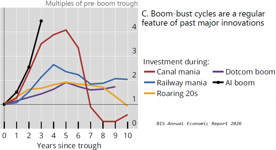
ORIGINAL CHART ANALYSIS — FROM MONDAY’S MIBBy year three, AI’s line has already cleared where Canal mania peaked in year five — the steepest curve of all five episodes, near 4.3x its trough and still climbing vertically, with railways, the Roaring Twenties, even the canals’ high behind it. That settles the “just another dotcom bubble” reflex: dotcom was the mildest episode here, cresting around 1.5x. But the reframing that matters isn’t the shape — it’s the letterhead. The Bank for International Settlements, the central banks’ bank, has formally entered AI capex into a two-century register of manias, each ending in reversal and recession, recategorizing it from an earnings story into a financial-stability one. And the reversal is the base case, not the tail: canals round-tripped to zero by year eight, the Roaring Twenties bled below their start, even railways and dotcom merely plateaued — none kept climbing. AI simply stops at year three, short of every inflection where the others rolled over. The mechanism decides which line it follows: over $1 trillion of hyperscaler capex is outrunning earnings and free cash flow, and whether returns arrive before that committed capital must be serviced sorts plateau from round-trip. First-order, markets reprice multiples and spreads; second-order, a capex bust drags GDP and jobs. AI’s worst chart is still blank.
MIB Weekly Digest Ver. 1.69
For professional investors only. Not investment advice.
© 2026 RecessionALERT.com
MIB Daily: Payrolls Miss (57K vs 115K) Fuels a Record Dow as Gold and Chips Flash a Warning — Can AI Capex Survive the Rotation Into Value?
MARKET INTELLIGENCE BRIEF (MIB)
Thursday, July 2, 2026
June payrolls badly missed at 57K vs. 115K est.; unemployment fell to 4.2% only as participation hit a five-year low. Dow rode Fed rate-cut hopes to a record (+1.14%) even as gold’s 1.3% jump read it as a growth warning. Semiconductors extended their rout (SanDisk -14%, KLA -11.5%) as Meta (-4.9%) admitted AI agents “hasn’t accelerated as expected.” Tesla fell 7.5% despite blowout deliveries; O’Reilly bid ~$10B for GPC’s NAPA; oil hit a 4-month low on US-Iran progress.
TABLE OF CONTENTS
A. EXECUTIVE SUMMARY
B. MARKET DATA
C. HIGH-IMPACT STORIES (6)
D. MODERATE-IMPACT STORIES (6)
E. ECONOMY WATCH (2)
F. EARNINGS WATCH (0)
G. WHAT’S NEXT
H. CHART OF THE DAY
A. EXECUTIVE SUMMARY -> TOP
Equities diverged sharply as June nonfarm payrolls badly missed at 57,000 versus 115,000 expected — the third consecutive weak labor print after Wednesday’s ADP miss and the Atlanta Fed’s cut of GDPNow to 1.2% — sending the Dow to a record close (+1.14%) on rotation into Financials and Communication Services while the Nasdaq sank 0.8-1.6% on an extending semiconductor selloff. The unemployment rate’s drop to 4.2% masked genuine deterioration: labor-force participation fell to 61.5%, its lowest since March 2021, a discouraged-worker dynamic rather than labor-market strength. Bond and commodity markets read the report as a growth warning rather than a Fed-relief rally — gold jumped 1.3% and the 2-year yield fell further even as equities cheered reduced hike odds — a “bad news is good news” split that leaves the underlying economic signal more troubling than the tape suggests. Breadth stayed narrow: gains concentrated in rate-sensitive value and healthcare names while small-caps and tech-heavy growth lagged, extending — not reversing — the AI-trade repricing’s second day.
• Dow +594.83 (+1.14%) to a record 52,900.07 on Financials/Communication Services rotation; S&P 500 flat (-0.01%) at 7,482.70; Nasdaq 100 -1.61%.
• June nonfarm payrolls: +57K vs. 115K expected, unemployment 4.2% (participation lowest since March 2021); September Fed hike odds erased, October still debated ahead of the July 28-29 FOMC.
• Semiconductor selloff extends to a second day: SMH -4.5%, SanDisk -14.13%, KLA -11.51%, Lam Research -10.19%, Marvell -9.84%; Nvidia relatively resilient (-1.4%).
• Meta -4.90% after Zuckerberg tells staff AI agent development “hasn’t accelerated as expected,” reversing Wednesday’s 8.85% AI-cloud rally; Apple +4.84% as a perceived “memory shock” haven within tech.
• Tesla -7.49% (worst day in nearly a year) despite blowout Q2 deliveries of 480,126 (+25% YoY, beat by ~74K units) — sell-the-news on a stretched ~421x P/E.
• O’Reilly submits ~$10B all-cash bid for GPC’s NAPA unit (GPC +13%, ORLY -5%); oil hits a 4-month low (WTI $67.54, Brent $70.66) on Qatar-brokered “positive progress” in US-Iran Hormuz talks.
1. “Bad News, Good News” Divergence Between Equities and Bonds/Gold — Equities read today’s payrolls miss as reducing Fed tightening risk, pushing the Dow to a record. But gold’s 1.3% rally and a further yield decline suggest bond and commodity markets are pricing the same data as a genuine growth warning, not just rate relief. With Atlanta Fed GDPNow now at 1.2% and three consecutive weak labor signals (ADP, payrolls, participation), the equity tape’s confidence may be underpricing growth-deceleration risk heading into the July 28-29 FOMC.
2. The AI-Capex Trade Is Repricing Structurally, Not Just Pulling Back — Semiconductors logged a second straight day of double-digit declines (KLA, Lam, SanDisk, Marvell all down 9-14%), and Meta’s own admission that AI agent development has lagged expectations reopened the unmonetized-capex critique a day after its AI-cloud story briefly quieted it. Nvidia’s relative resilience (-1.4%) suggests markets are differentiating GPU/training demand from equipment and memory demand — a distinction worth tracking into hyperscaler Q2 earnings.
3. Rotation Toward Rate-Sensitive Value Continues to Build — Financials, Healthcare, and Communication Services (ex-Meta) led again today, while Technology remains the sector laggard both on the day and for the month (-9.02%) despite its 34.60% 12-month lead. Falling yields (mortgage rates now at a seven-week low of 6.43%) and Chevron’s Wolfe Research upgrade on a structural Guyana free-cash-flow thesis both point the same direction: capital is favoring durable cash-flow visibility over momentum exposure as the AI trade cools.
B. MARKET DATA -> TOP
U.S. equities delivered a bifurcated session as June nonfarm payrolls badly missed at 57K vs. roughly 110K expected — released a day early ahead of Friday’s holiday — easing Fed-hike fears and sending the Dow to a fresh record (+1.14%) on Financials and Communication Services leadership, even as the Nasdaq 100 slid 1.61% on a sharp semiconductor selloff. SanDisk, KLA, Lam Research, and Marvell each fell 9-14% as the AI-memory “Parabolic 7” trade unwound on Meta cloud-capacity concerns and stretched valuations; Apple bucked the rout, gaining 4.84% on perceived insulation from the memory shock. Tesla dropped 7.49% in a classic sell-the-news reaction despite blowout Q2 deliveries of 480,126 units. Gold jumped over 2% and the dollar softened on the weak jobs print, while Treasury yields were little changed.
CLOSING PRICES – Thursday, July 2, 2026:
MAJOR INDICES
The Dow’s record close and NYSE Composite’s +0.93% gain mask a starkly narrow session — Nasdaq 100’s 1.61% slide on the chip selloff confirms this was tech-specific, not market-wide, weakness. Dow Theory bull confirmation extends into a second session as DJ Transportation notches a fresh 10-session high alongside the industrials. Over the past 10 sessions, the S&P 500 has edged out the Nasdaq 100 by roughly 2 points — a modest but building broadening rotation toward value and cyclicals.
| Index | Close | Change | %Move | Why It Moved |
|---|---|---|---|---|
| S&P 500 | 7,482.70 | -0.53 | -0.01% | Tech drag offset value rotation; finished roughly flat |
| Dow Jones | 52,900.07 | +594.83 | +1.14% | Fresh record close; Financials and Communication Services led |
| DJ Transportation | 22,015.10 | +55.30 | +0.25% | Tracked blue-chip strength; new 10-session high |
| Nasdaq 100 | 29,321.29 | -479.92 | -1.61% | Semiconductor/memory-chip selloff dragged mega-cap tech |
| Russell 2000 | 2,994.93 | -17.66 | -0.59% | Small-caps missed the blue-chip rotation |
| NYSE Composite | 23,957.08 | +219.90 | +0.93% | Broad-based strength confirms rally beyond mega-cap tech |
VOLATILITY & TREASURIES
VIX fell 2.71% even as Treasury yields barely moved — the June NFP miss (57K vs. ~110K expected, released early for the holiday) eased near-term Fed-hike odds without producing a large bond rally, a muted curve reaction relative to the size of the miss. DXY’s 0.50% slide and gold’s 1.30% jump suggest the dollar and precious metals treated today’s jobs print as more consequential than the Treasury curve did.
| Instrument | Level | Change | Why It Moved |
|---|---|---|---|
| VIX | 16.14 | -0.45 (-2.71%) | Eased as broad market absorbed tech-specific selloff |
| 10-Year Treasury Yield | 4.469% | -0.6 bps | June NFP badly missed (57K vs. ~110K est.), released a day early for the holiday |
| 2-Year Treasury Yield | 4.137% | -2.7 bps | Front-end led on Fed easing repricing after today’s NFP miss |
| US Dollar Index (DXY) | 100.86 | -0.50 (-0.50%) | Dollar softened on today’s NFP miss |
COMMODITIES
Gold and silver moved in lockstep (+1.30%, +1.54%) on dollar weakness tied to the soft jobs print, while copper sat flat — an industrial-demand read unmoved by the rate-cut repricing. Platinum’s 1.99% gain confirms broad precious-metals participation rather than a gold-specific haven bid. Bitcoin’s modest 1.22% gain tracked the day’s mild risk-on tone in blue-chips rather than decoupling on crypto-specific news.
| Asset | Price | Change | %Move | Why It Moved |
|---|---|---|---|---|
| Gold | $4,135.65/oz | $+53.25 | +1.30% | Today’s NFP miss lifted rate-cut bets, weighed on the dollar, and boosted haven demand |
| Silver | $61.440/oz | $+0.929 | +1.54% | Tracked gold higher on the same macro drivers |
| Copper | $6.1755/lb | $-0.0040 | -0.06% | Essentially flat; no distinct catalyst |
| Platinum | $1,631.80/oz | $+31.90 | +1.99% | Broad precious-metals bid alongside gold, silver |
| Bitcoin | $61,568.0 | $+741.0 | +1.22% | Tracked mild risk-on tone in blue-chips |
ENERGY
WTI and Brent were essentially unchanged, with Brent flat and WTI down a token 0.20% — a muted session with no distinct catalyst on either benchmark. Henry Hub natural gas likewise sat still (-0.37%), fully decoupled from Dutch TTF’s 2.90% gain, confirming the divergence is a European-specific supply dynamic rather than a global gas story.
| Asset | Price | Change | %Move | Why It Moved |
|---|---|---|---|---|
| Crude Oil (WTI) | $68.44/bbl | $-0.14 | -0.20% | Muted session; no distinct catalyst |
| Crude Oil (Brent) | $71.58/bbl | $0.00 | 0.00% | Unchanged; flat session |
| Natural Gas (Henry Hub) | $3.208/MMBtu | $-0.012 | -0.37% | Flat trading, decoupled from TTF’s gain |
| Natural Gas (Dutch TTF) | $14.75/MMBtu | $+0.42 | +2.90% | European gas firmed on regional supply dynamics |
S&P 500 SECTORS
Technology’s reversal is the standout: 2026’s 3-month (+26.43%) and 12-month (+34.60%) leader is now the day’s biggest laggard (-1.72%) and this month’s worst performer (-9.02%), as the memory-chip selloff hit the sector’s most richly-valued names. Healthcare, by contrast, leads across every horizon from today (+2.80%) through 12 months (+22.35%) — a rare across-the-board consistency signal amid otherwise rotating leadership.
| Sector | 1-Day | 1-Week | 1-Month | 3-Month | 6-Month | YTD | 12-Month |
|---|---|---|---|---|---|---|---|
| Healthcare | +2.80% | +5.30% | +13.19% | +11.29% | +6.69% | +7.35% | +22.35% |
| Consumer Defensive | +2.26% | +0.82% | +3.67% | +2.24% | +7.57% | +8.13% | +4.96% |
| Basic Materials | +2.09% | +0.66% | -7.07% | -2.96% | +9.42% | +10.53% | +34.32% |
| Utilities | +1.94% | -0.45% | +2.76% | -1.30% | +6.21% | +6.87% | +13.40% |
| Real Estate | +1.20% | +0.69% | +3.94% | +10.11% | +9.53% | +10.66% | +8.79% |
| Energy | +1.18% | -1.09% | -8.68% | -10.09% | +18.16% | +18.72% | +24.90% |
| Financial | +1.14% | +3.28% | +7.32% | +13.53% | +3.87% | +4.64% | +13.20% |
| Industrials | +0.23% | -0.06% | +3.43% | +11.47% | +18.12% | +19.26% | +26.73% |
| Consumer Cyclical | -0.72% | +4.06% | -2.01% | +5.57% | -4.99% | -4.24% | +4.46% |
| Communication Services | -0.81% | +4.55% | -2.39% | +8.11% | +0.33% | +0.82% | +20.67% |
| Technology | -1.72% | -0.35% | -9.02% | +26.43% | +17.75% | +18.63% | +34.60% |
TOP MEGA-CAP MOVERS:
GAINERS
| Company | Ticker | Close | Change | Why It Moved |
|---|---|---|---|---|
| Apple Inc | AAPL | $308.63 | +4.84% | Rebound buying plus perceived insulation from the memory-chip shock; AI roadmap optimism |
| Netflix Inc | NFLX | $77.65 | +4.66% | Led the Communication Services sector rally (XLC +2.4%) |
| AbbVie Inc | ABBV | $261.07 | +3.99% | Rode broad Healthcare sector leadership (sector +2.80%) |
| RTX Corp | RTX | $199.25 | +3.90% | Rode broader blue-chip/industrials rotation; no confirmed company-specific catalyst |
| Johnson & Johnson | JNJ | $263.04 | +3.57% | Healthcare sector strength |
DECLINERS
| Company | Ticker | Close | Change | Why It Moved |
|---|---|---|---|---|
| Sandisk Corp | SNDK | $1,745.00 | -14.13% | “Parabolic 7” AI-memory trade unwind on Meta cloud-capacity report, valuation concerns |
| KLA Corp | KLAC | $235.55 | -11.51% | Broad semiconductor-equipment selloff amid AI capex worries |
| Lam Research Corp | LRCX | $351.41 | -10.19% | Chip-equipment selloff alongside KLA; valuation reset |
| Marvell Technology Inc | MRVL | $245.29 | -9.84% | Part of the “Parabolic 7” AI/memory trade unwind |
| Tesla Inc | TSLA | $393.94 | -7.49% | Sell-the-news despite blowout Q2 deliveries (480,126, +25% YoY); stretched valuation, US demand concerns |
C. HIGH-IMPACT STORIES -> TOP
UNCERTAIN
1. June Nonfarm Payrolls Miss Badly at 57K vs. 115K Consensus — September Hike Off the Table, 2Y Yield Falls, Dow Hits Record on “Bad News, Good News”
The core facts:Nonfarm payrolls rose just 57,000 in June, badly missing the 115,000 Dow Jones consensus and decelerating sharply from May’s downwardly revised 129,000. The unemployment rate fell to 4.2% from 4.3%, but only because the labor force participation rate dropped to 61.5% — its lowest since March 2021. The 2-year Treasury yield fell 3.5 basis points to 4.13% and the 10-year edged up 1 basis point to 4.485%. Traders removed a September Fed hike from pricing, though CME FedWatch still shows a potential October move; gold jumped 2.03% on the print.
Why it matters:This was the week’s binary risk event, and it resolved decisively soft — the third consecutive weak labor signal after Wednesday’s ADP miss (98K) and the Atlanta Fed’s slash of GDPNow to 1.2%. The falling participation rate masks the softness behind an artificially lower unemployment rate, a discouraged-worker dynamic rather than genuine labor strength. Equities read the report as reducing near-term Fed tightening risk (Dow to a fresh record), while gold’s rally signals bond/commodity markets are treating it as a genuine growth warning — a “bad news is good news” split that leaves the underlying economic signal more concerning than the equity tape suggests.
What to watch:CME FedWatch’s October hike probability heading into the July 28-29 FOMC meeting (a hike there is not expected); July’s employment report in early August for confirmation this is a genuine slowdown rather than a one-off print.
BULLISH
2. Dow Rips to Record Close (+594.83, +1.14%) as Weak Jobs Data Fuels Rotation Into Financials and Communication Services
The core facts:The Dow Jones Industrial Average gained 594.83 points (+1.14%) to a record close of 52,900.07, touching a fresh intraday high of 52,903.85, as easing Fed-hike fears from the weak jobs report drove rotation into Financials (XLF +2.2%) and Communication Services (XLC +2.4%). The S&P 500 was essentially flat, up less than a point to 7,483.24, while the Nasdaq Composite fell 0.8% to 25,832.67 as semiconductors dragged; the Russell 2000 underperformed, down 0.39%.
Why it matters:The sharp divergence between the record-setting Dow and the tech-heavy Nasdaq signals a genuine rotation rather than a broad risk-on rally — capital moved out of the red-hot AI/semiconductor trade that led H1 2026 and into rate-sensitive value names as bond yields eased. Combined with today’s semiconductor selloff, this is the clearest evidence yet that the AI-momentum trade is undergoing a real repricing rather than a one-day pullback, with small-caps (Russell 2000) also lagging as a sign of narrowing breadth.
What to watch:Whether Financials/Communication Services leadership persists into next week’s post-holiday session; continued Russell 2000 underperformance as a market-breadth signal.
BEARISH
3. Semiconductor Selloff Extends to a Second Day — SMH -4.5%, Teradyne -13.6%, KLA -11.5%, as Meta’s AI Doubts Compound the Chip-Cycle Rout
The core facts:The VanEck Semiconductor ETF (SMH) fell 4.5% for a second consecutive session, led by Teradyne -13.6%, KLA -11.5%, and Micron -5.5%, while Nvidia held up relatively better at -1.4%. This extends the multi-day “Parabolic 7” unwind that began June 30-July 1 (KLAC, MU, SNDK, AMAT, LRCX were already down double digits), originally triggered by Meta’s reported plans for a standalone AI cloud business to sell excess compute, and compounded today by Applied Materials CEO Gary Dickerson’s disclosed $14.7M insider stock sale.
Why it matters:This is now a two-day, multi-name structural correction in the sector that led the market through H1 2026 (SMH +82% in H1), not an isolated single-stock event. Nvidia’s relative resilience continues to suggest markets are differentiating GPU/AI-training demand (still intact) from equipment and memory demand (now in question amid hyperscaler self-sufficiency concerns). Today’s fresh catalyst — Meta CEO Zuckerberg’s own admission that AI agent development “hasn’t accelerated as expected” — adds a second, independent data point casting doubt on near-term AI monetization pace, reinforcing rather than reversing the selloff.
What to watch:Whether Nvidia’s relative outperformance persists as the GPU-vs-memory demand differentiator; hyperscaler capex commentary ahead of Q2 earnings in late July.
UNCERTAIN
4. O’Reilly Automotive Submits ~$10B All-Cash Bid for Genuine Parts’ NAPA Unit — GPC +13%, ORLY -5%
The core facts:O’Reilly Automotive submitted an all-cash bid valued at $10 billion or more for Genuine Parts Company’s NAPA auto-parts arm, according to a Bloomberg report. GPC has been working with JPMorgan Chase and Guggenheim Securities since February to separate its auto-parts business and become a pure-play industrial distributor. A completed deal would be O’Reilly’s largest since its 2008 acquisition of CSK Auto Corp for roughly $1 billion. GPC shares jumped 13%; ORLY fell 5% on deal-size and financing concerns.
Why it matters:The deal would meaningfully consolidate the automotive aftermarket-parts industry, bringing NAPA — one of the sector’s most recognized brands — under O’Reilly’s ownership while allowing GPC to pursue a cleaner, industrials-only profile. ORLY’s decline reflects investor concern over financing size and integration risk for a deal roughly ten times the size of its largest prior acquisition; GPC’s surge reflects both the premium implied by an all-cash offer and validation of its industrials-focused pivot announced in February.
What to watch:Formal deal confirmation and financing structure — this remains an unconfirmed report, not an announced transaction; potential competing bidders in what is described as an active auction process.
BEARISH
5. Oil Slides to 4-Month Low as Qatar Reports “Positive Progress” in US-Iran Hormuz Talks — WTI $67.54, Brent $70.66
The core facts:Brent crude fell $0.91 (-1.3%) to $70.66/barrel and WTI fell $1.04 (-1.5%) to $67.54/barrel — both the lowest levels since late February 2026, just before the US-Israel-Iran conflict began. The decline followed Qatar’s confirmation that US and Iranian negotiators made “positive progress” in Doha talks tied to the ceasefire memorandum, easing fears of renewed Strait of Hormuz disruption. Qatar’s Foreign Ministry noted no breakthrough yet toward a lasting peace; the next meeting is scheduled after July 9 funeral processions for Iran’s late Supreme Leader.
Why it matters:This marks a genuine turn from Tuesday’s setback (Iran declining scheduled talks) back toward diplomatic progress, extending the multi-week unwind of the war-risk premium built into oil prices since the conflict began. Combined with the EIA’s confirmed pattern of crude-inventory draws failing to support prices, the move confirms the structural 2026 oversupply thesis (JPMorgan/Citi ~4M bbl/day surplus) remains the dominant price driver over both supply-disruption risk and inventory data. Falling energy costs are modestly disinflationary at the margin — a small tailwind against the Fed’s “prices too high” concern — but a continued headwind for energy-sector earnings.
What to watch:The post-July 9 resumption of US-Iran talks for signs of durable normalization versus renewed stalemate; WTI’s test of the ~$67 February 2026 low as technical support.
BEARISH
6. Meta Falls 4.90% as Zuckerberg Tells Staff AI Agent Development “Hasn’t Accelerated as Expected” — Reverses Wednesday’s AI-Cloud Rally
The core facts:Meta shares fell 4.90% Thursday after CEO Mark Zuckerberg told employees in an internal town hall that AI agent development “hasn’t accelerated in the way we expected” over the past four months — a sharp reversal from Wednesday’s 8.85% surge on reports of a standalone AI cloud business. The remarks come as Meta has raised full-year 2026 capex guidance to $125-145 billion (from $115-135 billion) to fund AI infrastructure, and follow May layoffs tied to AI restructuring that have yet to produce the anticipated results.
Why it matters:The reversal directly undercuts Wednesday’s bullish reframing of Meta’s AI spend as a monetizable cloud-revenue opportunity — Zuckerberg’s own admission that internal agent development is lagging expectations reopens the core investor critique (unmonetized, escalating capex with an uncertain payoff timeline) that Wednesday’s cloud-business report had briefly quieted. Communication Services had been the week’s best-performing sector on AI-cloud optimism; today’s reversal, paired with the ongoing semiconductor selloff, suggests markets are broadly re-examining AI-capex return timelines across both chip suppliers and hyperscalers simultaneously.
What to watch:Meta’s Q2 2026 earnings call (expected late July) for management’s formal framing of AI agent progress and capex ROI; peer hyperscaler commentary on AI agent monetization timelines.
D. MODERATE-IMPACT STORIES -> TOP
UNCERTAIN
7. Tesla Falls 7.49% — Worst Day in Nearly a Year — Despite Blowout Q2 Deliveries of 480,126 Vehicles, +25% YoY
The core facts:Tesla delivered 480,126 vehicles in Q2 2026, up 25% year-over-year and well above Wall Street’s roughly 406,600 consensus — a beat of approximately 74,000 units; energy storage deployments reached 13.5 GWh versus 13.3 GWh expected. Despite the decisive beat, TSLA shares fell approximately 7.49%, the stock’s worst single day in nearly a year, in a “sell the news” reaction after a 13%+ run into the report. Tesla reports full Q2 2026 financial results after market close on July 22.
Why it matters:The negative reaction to a decisive delivery beat signals investors have shifted focus from unit volumes to profitability — Tesla’s rich ~421x P/E multiple had already priced in the beat and more, leaving no room for a “sell the news” outcome even on strong operational execution. Today’s broader risk-off tone in high-multiple growth names (semiconductor selloff, weak jobs data) compounded the move. The real test shifts to the July 22 earnings report, where margins and US demand trends post-EV-tax-credit-expiration will determine whether delivery strength translates into earnings support for the valuation.
What to watch:Tesla’s July 22 Q2 2026 earnings report for gross margin trends and US demand commentary following the EV tax credit expiration.
BULLISH
8. Apple Rallies 4.84% as Investors Frame It a “Memory Shock” Safe Haven Within Tech
The core facts:Apple shares rose 4.84% even as the broader semiconductor/memory complex sold off sharply for a second consecutive session, with commentary framing Apple as relatively insulated from rising memory-chip input costs given its diversified supply chain and pricing power. The move also reflects rebound buying following a June 25 pullback tied to reports of Mac/iPad price increases.
Why it matters:Apple’s outperformance against a collapsing semiconductor tape signals investors are differentiating between companies exposed to rising component costs (memory/equipment makers now facing both an HBM/DRAM repricing and hyperscaler self-sufficiency concerns) and large-cap consumer technology names seen as able to pass through or absorb higher input costs. The move reinforces the day’s broader “Great Rotation” theme — capital shifting away from AI-infrastructure-exposed names toward companies perceived as further from the center of the memory-chip cost shock.
What to watch:Formal confirmation of Mac/iPad price increases tied to rising memory costs; whether Apple sustains the rebound if the semiconductor selloff persists into next week.
BULLISH
9. 30-Year Mortgage Rate Falls to Seven-Week Low of 6.43% as Bond Yields Ease on Weak Jobs Data
The core facts:Freddie Mac’s weekly Primary Mortgage Market Survey showed the average 30-year fixed mortgage rate fell to 6.43% for the week ended July 2, down from 6.49% the prior week — the lowest level in seven weeks, since May 14’s 6.36%. The decline tracks the broader bond-yield retreat following today’s weak June jobs report.
Why it matters:Modestly lower mortgage rates provide incremental relief for housing affordability at the margin, with Realtor.com noting pending home sales have now risen for seven consecutive months. The move is a direct market-impact extension of today’s jobs-driven bond rally — as the 2-year Treasury yield fell 3.5 bps on reduced Fed hike odds, mortgage-linked rates eased in tandem, illustrating the labor-market-to-housing transmission channel the Fed’s rate path directly influences.
What to watch:Whether the rate decline persists through the July 4 holiday week and translates into a pickup in the weekly MBA purchase application index.
BULLISH
10. Nvidia Launches Revenue-Sharing “DSX AI Factory” Program to Widen AI-Startup Cloud Access
The core facts:Nvidia rolled out a “DSX AI Factory” partnership program giving AI-native cloud providers access to its infrastructure through revenue-sharing and credit-backed financing — rather than requiring full cash payment upfront, Nvidia collects standard hardware revenue plus a recurring share of resulting cloud income, while offering buyback guarantees on unsold GPU capacity. Early named partners Sharon AI (up to 40,000 GB300 GPUs in Australia) and Firmus Technologies (Indonesia) represent a combined potential deployment of up to 210,000 GPUs; Nvidia named Baseten, Fireworks AI, and Together AI as the type of AI-native customer the program targets.
Why it matters:The financing structure shifts Nvidia from a pure equipment vendor toward a financier with a direct stake in customer utilization, lowering the capital barrier for smaller AI-native cloud providers and reducing their dependency on hyperscalers building proprietary chips. Diversifying Nvidia’s customer base toward smaller AI-native buyers is a structurally defensive move at a moment when today’s session raised fresh questions — via Meta’s cloud-business plans and AI-agent-pace remarks — about the durability of hyperscaler GPU demand.
What to watch:Additional partner announcements under the DSX program; whether the revenue-sharing model becomes a template other GPU/chip suppliers adopt to defend market share.
BULLISH
11. Lockheed Martin +4.62% as It Emerges as Frontrunner for Ultra Maritime in ~$3.5B Naval-Tech Deal
The core facts:Lockheed Martin shares rose 4.62% after a Financial Times report identified the company as the frontrunner to acquire Ultra Maritime, a naval anti-submarine warfare technology specialist and division of Advent’s Cobham Ultra business, in a deal that could be valued around $3.5 billion. No formal agreement has been reached and several other bidders remain in the competitive auction process; a public announcement could come as soon as next week.
Why it matters:Ultra Maritime’s sonobuoy and anti-submarine detection technology would be a differentiated addition to Lockheed’s naval defense portfolio amid elevated global defense spending. The deal, while not yet finalized, would rank among Lockheed’s larger recent acquisitions and signals continued consolidation appetite in the defense-technology supply chain; the stock’s reaction reflects market approval of the strategic rationale, though the outcome remains contingent on the competitive bid process.
What to watch:Formal deal confirmation, expected as soon as next week; the final agreed price relative to the reported $3.5 billion figure amid a competitive bidding process.
BULLISH
12. Chevron Upgraded to Outperform at Wolfe Research — $210 Price Target Implies 27% Upside on Guyana Free-Cash-Flow Inflection
The core facts:Wolfe Research upgraded Chevron to “Outperform” from “Peer Perform” with a $210 price target, implying roughly 27% upside from Wednesday’s $165.69 close. The firm cited a share-price pullback since the start of the year that has masked improving long-term free-cash-flow prospects, including incremental production options secured since January that extend the FCF growth outlook beyond 2030, and a pending inflection in Guyana free cash flow — the first since the Hess acquisition closed in July 2025.
Why it matters:The upgrade comes even as crude prices fell to a 4-month low today, underscoring that Wolfe’s thesis is structural — long-duration FCF growth from Guyana and other production additions — rather than a near-term commodity-price call, a distinction relevant for energy investors weighing today’s bearish oil-price action against company-specific fundamentals. Chevron shares outperformed the broader energy complex despite falling oil prices, suggesting the market is beginning to price in the FCF inflection thesis independent of spot crude direction.
What to watch:Chevron’s Q2 2026 earnings report for early confirmation of the Guyana FCF inflection; further sell-side commentary following Wolfe’s upgrade.
E. ECONOMY WATCH -> TOP
June payrolls rose just 57,000 — roughly half the 115K consensus — with April-May revised down a net 74,000 and unemployment’s dip to 4.2% explained by a shrinking, not strengthening, labor force (participation fell to a five-year low of 61.5%). The miss reset rate expectations fast: the 2-year Treasury yield dropped 5+ bps and traders now see little room for a July Fed hike, a reversal from Wednesday’s hawkish-leaning Warsh commentary. That yield relief immediately fed through to housing, where the 30-year mortgage rate slid to a seven-week low of 6.43%, extending a fourth straight weekly decline. GDPNow still holds at 1.2% for Q2 — the weakest since 2023 — with markets now betting the Fed blinks before growth does.
June Payrolls Add Just 57,000, Badly Missing 115K Estimate as Unemployment Rate Dips to 4.2% on Shrinking Labor Force (BLS, July 2, 2026)
What they’re saying:Nonfarm payrolls rose a seasonally adjusted 57,000 in June, roughly half the 115,000 Dow Jones consensus and down sharply from May’s downwardly revised 129,000. April and May were revised down a combined net 74,000. Government payrolls added just 8,000 versus a 32,000 prior gain, and household employment fell by 507,000. Average hourly earnings rose 0.3% MoM and 3.5% YoY, both in line with estimates — meaning real wage growth continues to track below inflation for a third straight month.
The context:The unemployment rate ticked down to 4.2% from 4.3%, a mild surprise versus the 4.3% consensus, but the improvement was driven by a 0.3-point drop in labor force participation to 61.5% — the lowest since March 2021 — meaning fewer people looking for work rather than more people finding it. JPMorgan Asset Management’s David Kelly called the report a “reality check for the real economy,” describing a “tortoise” economy of sluggish growth. The 2-year Treasury yield fell more than 5 bps to 4.108% as traders sharply pared bets on a July Fed hike, with one strategist noting it is now “difficult to envision a path toward a July Fed hike.”
What to watch:FOMC meeting July 28-29 — markets will watch whether Chair Warsh’s “inflation too high” stance from Wednesday’s ECB Forum remarks holds against a visibly cooling labor market. Next jobs report (July NFP) due August 7.
30-Year Mortgage Rate Falls to 6.43%, Seven-Week Low, as Bond Yields Retreat on Weak Jobs Data (Freddie Mac, July 2, 2026)
What they’re saying:The average 30-year fixed mortgage rate fell to 6.43% this week, down from 6.49%, marking its lowest level in seven weeks and a fourth consecutive weekly decline. The 15-year rate eased to 5.79% from 5.84%.
The context:The drop tracks the retreat in Treasury yields following today’s weak June jobs report, which reduced the odds of a near-term Fed rate hike. Realtor.com chief economist Danielle Hale pointed to eight consecutive months of declining home prices and seven months of gains in pending home sales as evidence buyers — mainly higher-income — are adjusting to the mid-6% rate environment as the “new normal,” with purchase demand edging higher.
What to watch:Weekly MBA mortgage applications data for confirmation that lower rates are translating into purchase activity; existing home sales data expected mid-July.
F. EARNINGS WATCH -> TOP
YESTERDAY AFTER THE BELL (Markets Reacted Today)
No major earnings yesterday after the bell from companies with >$100B market cap.
TODAY BEFORE THE BELL (Markets Already Reacted)
No major earnings before the bell from companies with >$100B market cap. (Lindsay Corp and Greenbrier Companies reported BMO but both remain well under the $100B threshold.)
TODAY AFTER THE BELL (Markets React Tomorrow)
No major earnings after the bell from companies with >$100B market cap.
WEEK AHEAD PREVIEW:
Markets are closed Friday, July 3 for Independence Day. Q1 2026 earnings season is effectively complete (89% reported); Q2 2026 season opens in earnest the week of July 6-10, with the next FactSet scorecard update due ~July 11.
PepsiCo (PEP) — BMO, Thursday July 9 — Consensus calls for $2.21 EPS on $23.96B revenue. Key focus: continued weakness at PepsiCo Foods North America and whether management signals the recovery timeline slipping further into H2, versus continued international strength (5.4% organic sales growth expected).
No other >$100B US-domiciled reporters are confirmed for Monday-Wednesday (July 6-8); Q2 2026 earnings season begins in earnest with PepsiCo’s report.
G. WHAT’S NEXT -> TOP
UPCOMING RELEASES:
| Date | Event | Why It Matters |
|---|---|---|
| Mon, Jul 6 | ISM Services PMI (prior 54.5) | Gauges service-sector momentum; a further slowdown here alongside today’s weak payrolls would reinforce the “tortoise economy” narrative and build the case for near-term Fed easing. |
| Tue, Jul 7 | Balance of Trade (prior -$55.9B) | Trade-deficit trends feed directly into GDP tracking estimates already under pressure, with Atlanta Fed GDPNow at 1.2%. |
| Tue, Jul 7 | Consumer Inflation Expectations (prior 3.5%) | Tests whether softening labor data is bleeding into inflation psychology — a key input to the Fed’s July 28-29 policy debate. |
| Wed, Jul 8 | FOMC Minutes | Markets will parse how seriously the Fed weighed today’s payrolls miss against Chair Warsh’s “inflation too high” stance from this week’s ECB Forum remarks. |
| Wed, Jul 8 | Consumer Credit Change (prior $20.73B) | Signals household borrowing appetite amid a cooling labor market and easing mortgage rates. |
KEY QUESTIONS:
1. Does the June payrolls miss mark the start of a genuine labor-market slowdown or a one-off print — and will the July 28-29 FOMC treat it as license to cut, given Chair Warsh’s “inflation too high” stance just two days earlier?
2. Is the semiconductor/AI-capex selloff a healthy repricing of a crowded trade or the start of a broader unwind — does Nvidia’s relative resilience hold once hyperscaler Q2 earnings arrive?
3. Does the O’Reilly-GPC NAPA bid finalize as reported, and does Qatar’s “positive progress” on US-Iran Hormuz talks translate into durable de-escalation once negotiations resume after July 9?
H. CHART OF THE DAY -> TOP
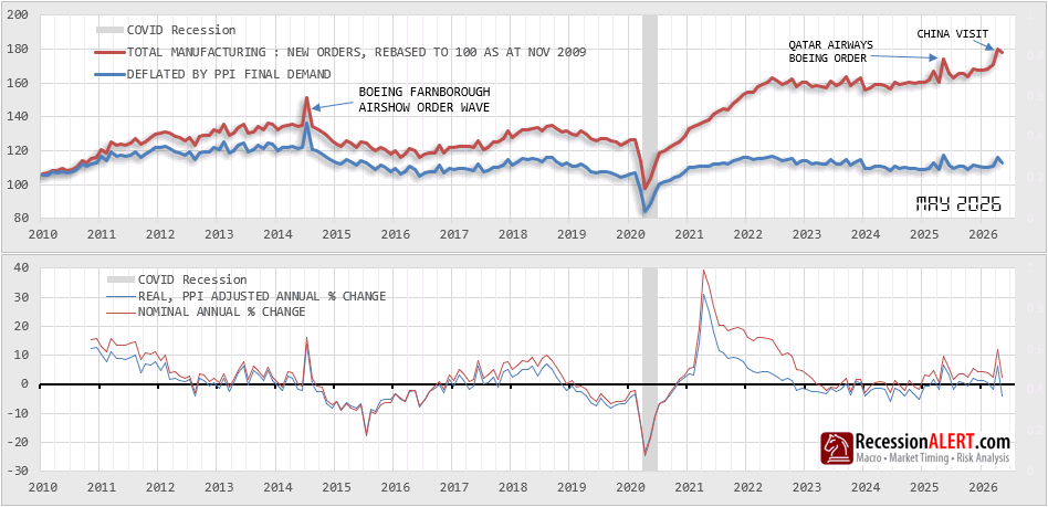
The record is a mirage, and the annotations show the wires. Nominal manufacturing new orders just hit an all-time high — 180.2 in April, 177.9 in May on a November-2009=100 base — yet deflate the same series by PPI Final Demand and real order volume sits at just 113. Sixty-five points of price, thirteen of volume. Two forces build the gap. The first is cumulative producer-price inflation — fifteen years of it — the entire structural wedge between the lines. The second is lumpier: the sharpest moves to the highs are Boeing order events, not broad demand — the 2014 Farnborough wave, Qatar Airways in 2025, and the mix of large widebody orders and a China deal propping up this spring’s record itself. A handful of aircraft contracts, booked in the most volatile category in the series, is doing the work the headline credits to manufacturing. Strip the deflator and the planes, and real orders have flatlined for fifteen years, below their 2013 peak. Feed a leading index the nominal line and it reads a state-visit aircraft order as an economic upturn — the number your model should ignore. Ingest this factor in real terms, as RecessionAlert’s US Monthly Leading Index does, or not at all.
Market Intelligence Brief (MIB) Ver. 18.42
For professional investors only. Not investment advice.
© 2026 RecessionALERT.com
MIB Daily: META +8.85% threatens the chip trade from within (SOX -7%) — short semis, own Financials as Thursday’s NFP decides the stagflation exit
MARKET INTELLIGENCE BRIEF (MIB)
Wednesday, July 1, 2026
META +8.85% on AI cloud reports; global semi selloff (KLAC -11.8%, MU -10.57%, SOX -7%) split Q3’s opening session. Atlanta Fed cut GDPNow to 1.2% from 2.5% — 2026’s largest single-day revision — as ADP missed at 98K; Thursday’s NFP is the binary risk event. Warsh at ECB Sintra refused July guidance with hike odds at 54%; 10Y +6 bps to 4.48%. WFC +3.99% on Goldman upgrade and 11% dividend raise as all 32 banks cleared stress tests; Financials +1.61%.
TABLE OF CONTENTS
A. EXECUTIVE SUMMARY
B. MARKET DATA
C. HIGH-IMPACT STORIES (5)
D. MODERATE-IMPACT STORIES (5)
E. ECONOMY WATCH (6)
F. EARNINGS WATCH (0)
G. WHAT’S NEXT
H. CHART OF THE DAY
A. EXECUTIVE SUMMARY -> TOP
Q3 2026 opened on a split screen: META’s AI cloud business announcement — transforming $50B+ in unmonetized capex into a revenue stream competing with AWS, Azure, and Google Cloud — drove Communication Services to the session’s top sector (+2.61%), while a global semiconductor selloff (KLAC -11.8%, MU -10.57%, SOX -7%) pushed the Nasdaq 100 down -1.54% against a flat Dow. The macro backdrop darkened simultaneously: Atlanta Fed GDPNow collapsed from 2.5% to 1.2% — the largest single-day revision of 2026 — as ADP missed at 98K and the 10-year yield rose 6 bps to 4.48% after Fed Chair Warsh refused any July rate guidance at the ECB Sintra forum. VIX gained only 0.73% despite tech’s rout, confirming orderly selling — but Q3 begins with a stagflationary backdrop: growth at 1.2%, inflation “too high” by Warsh’s own declaration, and no Fed backstop.
• META +8.85% on Bloomberg reports of a new AI cloud business to sell compute and models externally; Communication Services best sector (+2.61%); PLTR +7.73% on enterprise AI beneficiary sentiment; META added ~$130B in market cap in a single session.
• Global semiconductor rout: KLAC -11.8%, MU -10.57%, SNDK -10.50%, AMAT -9.97%, LRCX -9.71%; SOX opened -7%; KOSPI circuit breaker triggered in Asia. Technology worst S&P 500 sector at -2.35% — reversing its YTD leadership (+20.71%).
• Atlanta Fed GDPNow cut to 1.2% from 2.5% — the largest single-day revision of 2026 — after ADP June payrolls came in at 98K (vs. 113K consensus), the softest since late 2025. Thursday’s BLS Nonfarm Payrolls (consensus 110K, Pantheon 75K, prior 172K) is the week’s binary risk event.
• Warsh declines July guidance at ECB Sintra forum; July hike odds remain at 54%; 10Y rose 6 bps to 4.48%; no safe-haven Treasury bid. Utilities -1.38%, Industrials -2.28% as rate-sensitive sectors absorbed the higher-for-longer signal.
• WFC +3.99% on Goldman Sachs Conviction List addition and 11% dividend raise ($0.50/share Q3); all 32 banks cleared the 2026 Fed stress test; Financials +1.61%, second-best sector. JPMorgan and Goldman also announced capital returns.
• ISM Manufacturing Prices Paid -9.1 pts to 73.0 — largest single-month drop since July 2022; WTI -1.99% to $68.12 (2026 low) despite EIA 3.8M barrel crude draw; Goldman cuts 12-month US recession odds to 15%, citing Iran peace deal energy relief.
1. AI monetization fractures the chip trade — META’s pivot to an external cloud business simultaneously validates AI infrastructure investment and raises hyperscaler self-sufficiency risk, threatening addressable demand for third-party chip vendors. SK Hynix’s deliberate HBM4 slowdown — redirecting capacity to conventional DRAM where margins now exceed HBM premiums — confirms the demand inflection at the supply side itself. The 82% H1 SOX gain embedded the most optimistic scenario; today’s 7% single-session correction is the first real stress test of the AI capex supercycle thesis entering Q3.
2. Stagflation re-emerges as Q3’s defining portfolio tension — Today’s synchronized signals — GDPNow at 1.2%, ADP at 98K, ISM Prices Paid plunging 9.1 points, Warsh declining any guidance — construct the rarest investing environment: slowing growth, inflation “too high” by the Fed Chair’s own declaration, and a central bank explicitly without a policy backstop. The 10Y rising 6 bps while equities fell (no safe-haven bond bid) confirms markets are not treating decelerating growth as a bullish-for-bonds signal. Thursday’s NFP is the critical test of whether the labor market confirms this deterioration or provides a reprieve before the July 16–17 FOMC.
3. Financials as the structural rotation anchor — Banks entering Q3 fully capitalized (all 32 cleared stress tests), raising dividends, and positioned for NIM expansion in a higher-for-longer rate environment offer the clearest defensive growth trade in a stagflationary backdrop. Goldman’s Conviction List addition of WFC signals the bank upgrade cycle is early-stage; the OCC asset cap removal — not yet priced — remains the next major re-rating catalyst. On a day when the broad market drifted and tech sold off, Financials’ +1.61% session performance signals institutional rotation toward rate-beneficiary names as Q3’s inflation-hedge anchor.
B. MARKET DATA -> TOP
The opening session of Q3 2026 delivered a stark bifurcation: Meta Platforms surged 8.9% on Bloomberg reports of a new external AI cloud business — answering investor AI-capex ROI concerns — catapulting Communication Services (+2.61%) to the day’s top sector, while semiconductor equipment names (KLA -11.8%, Applied Materials -9.97%) deepened June’s chip-cycle sell-off and dragged Technology to -2.35%. The Nasdaq 100 fell -1.54% while the Dow barely moved (-0.02%) and DJ Transports gained +0.97% on crude’s continued slide, revealing a narrow, sector-specific rout beneath a resilient market surface. Wells Fargo jumped 3.99% after clearing the 2026 Fed stress test and raising its dividend 11%. The 10-year yield rose 6 bps to 4.48% as Fed Chair Warsh offered no rate guidance at the global central bank panel.
CLOSING PRICES – Wednesday, July 1, 2026:
MAJOR INDICES
The Nasdaq 100’s -1.54% loss against the Dow’s near-flat close (-0.02%) defines the day: this was a tech/semi rout, not a broad selloff. Russell 2000 (-0.30%) and NYSE (-0.41%) confirm the damage was concentrated. Dow Theory bull confirmation emerges today (first session): both DJIA and DJTA are within 1.1% of their 10-session highs. Russell 2000 has outpaced the S&P 500 over the trailing 10 sessions by 2.83% — an entrenched broad-participation pattern now in its 10th consecutive session.
| Index | Close | Change | %Move | Why It Moved |
|---|---|---|---|---|
| S&P 500 | 7,483.40 | -15.96 | -0.21% | Mixed session — META AI cloud story lifted Communication Services; semiconductor equipment rout dragged Technology -2.35%; net modest decline |
| Dow Jones | 52,306.22 | -12.98 | -0.02% | Virtually flat; blue-chip index absorbed the tech selloff while Financials and Consumer Cyclical added support |
| DJ Transportation | 21,959.7 | +209.9 | +0.97% | Crude oil fell -2%; lower fuel-cost expectations lifted freight and logistics names heading into Q3 |
| Nasdaq 100 | 29,809.13 | -467.22 | -1.54% | Semiconductor equipment names (KLA -11.8%, Micron -10.6%, Applied Materials -9.97%) led a concentrated chip-cycle sell-off dominating the tech-heavy index |
| Russell 2000 | 3,015.34 | -9.03 | -0.30% | Modest decline in a mixed session; small-cap broad-participation signal intact over 10-session window vs S&P 500 |
| NYSE Composite | 23,737.18 | -97.05 | -0.41% | Mixed breadth — 5 of 11 sectors gained, 6 declined; rotation from Technology into Communication Services and Financials |
VOLATILITY & TREASURIES
VIX rose just 0.73% despite the Nasdaq’s -1.54% decline — orderly selling, not panic. The 10Y jumped 6 bps to 4.48% while equities fell, with bonds declining to bid; Fed Chair Warsh offered no rate-cut signals at the global central bank panel, stranding the market without a policy backstop. The 10Y rising 6 bps vs the 2Y’s 3.7 bps steepens the curve modestly — a subtle reflationary tilt as Q3 begins.
| Instrument | Level | Change | Why It Moved |
|---|---|---|---|
| VIX | 16.57 | +0.12 (+0.73%) | Modest uptick on tech/semi declines; muted fear response signals selling is orderly; well below systemic-concern levels |
| 10-Year Treasury Yield | 4.482% | +6.0 bps | Fed Chair Warsh offered no rate-cut guidance; bonds declined alongside equities — no safe-haven flight to Treasuries despite equity weakness |
| 2-Year Treasury Yield | 4.176% | +3.7 bps | Short-end yields rose less than 10Y; modest curve steepening signal; markets not pricing near-term Fed action |
| US Dollar Index (DXY) | 101.39 | +0.20 (+0.20%) | Mild dollar strength on lack of Fed dovish guidance; DXY consolidating after Q2 softness |
COMMODITIES
Gold +0.31% while silver fell -0.36% — a minor precious metals split signaling mild safe-haven positioning; platinum’s +1.35% aligns with gold, not industrial metals. Copper’s -1.54% decline echoes the semiconductor capex-cycle concern narrative and a soft industrial demand backdrop. Bitcoin’s +2.05% decoupled from a broadly lower equity tape, testing the $60K threshold — crypto-specific positioning rather than risk sentiment.
| Asset | Price | Change | %Move | Why It Moved |
|---|---|---|---|---|
| Gold | $4,050.85/oz | +$12.35 | +0.31% | Mild safe-haven bid amid equity uncertainty; gold holding above $4,000 psychological level; rising yield pressure limits upside |
| Silver | $59.708/oz | -$0.214 | -0.36% | Industrial demand concerns weigh; diverging from gold reflects risk-off rather than inflation-hedge buying |
| Copper | $6.1575/lb | -$0.0965 | -1.54% | Soft industrial demand signal; decline aligns with semiconductor capex concerns and mixed global growth outlook |
| Platinum | $1,586.90/oz | +$21.10 | +1.35% | Moving with gold in safe-haven mode; autocatalyst demand steady; diverging from copper’s industrial weakness |
| Bitcoin | $59,979 | +$1,203 | +2.05% | Decoupled from equity weakness; crypto-specific positioning as BTC tests the $60K threshold; not tracking risk sentiment today |
ENERGY
WTI (-1.99%) and Brent (-2.34%) fell in near-identical lockstep — no spread widening — confirming a global demand and supply-dynamics story, not a regional disruption. Iran’s rejection of direct US talks failed to add a geopolitical premium; markets are pricing improved supply availability over political risk. Natural gas fell -2.26% alongside crude — broad energy deflation. Oil declining with equities signals soft demand expectations, not a supply shock.
| Asset | Price | Change | %Move | Why It Moved |
|---|---|---|---|---|
| Crude Oil (WTI) | $68.12/bbl | -$1.38 | -1.99% | Q2 2026’s largest quarterly crude decline since 2020 (~30% Q2 drop) carries into Q3; demand concerns outweigh Iran diplomatic tensions |
| Crude Oil (Brent) | $71.24/bbl | -$1.71 | -2.34% | Iran rejected direct US talks but market focused on demand weakness and OPEC supply dynamics; global benchmark extending June losses |
| Natural Gas (Henry Hub) | $3.201/MMBtu | -$0.074 | -2.26% | Broad energy complex weakness; mild Q3 seasonal demand outlook; moving in tandem with crude |
| Natural Gas (Dutch TTF) | $14.26/MMBtu | -$0.28 | -1.90% | European gas declining with US; Iran nuclear uncertainty reduced supply-risk premium; TTF/Henry Hub moving in tandem today |
S&P 500 SECTORS
Today’s headline divergence: Communication Services surged +2.61% on META’s cloud announcement yet sits -3.84% over the past month — a sharp single-day reversal of June’s laggard. Technology is today’s worst sector (-2.35%) despite leading YTD (+20.71%) and the 3-month period (+30.14%); the semi equipment rout corrects an historically extended run. Industrials’ session loss (-2.28%) stands out against +18.86% YTD strength — lower oil helps Transports, but broader industrial stocks face yield-pressure headwinds.
| Sector | 1-Day | 1-Week | 1-Month | 3-Month | 6-Month | YTD | 12-Month |
|---|---|---|---|---|---|---|---|
| Communication Services | +2.61% | +4.32% | -3.84% | +10.51% | +1.45% | +1.66% | +20.35% |
| Financial | +1.61% | +2.05% | +6.50% | +12.87% | +2.52% | +3.47% | +12.53% |
| Consumer Cyclical | +0.87% | +3.16% | -1.64% | +7.21% | -4.69% | -3.52% | +5.40% |
| Real Estate | +0.37% | -0.23% | +3.16% | +9.18% | +8.47% | +9.37% | +8.22% |
| Healthcare | +0.22% | +3.87% | +8.47% | +9.22% | +3.40% | +4.43% | +20.23% |
| Consumer Defensive | -0.49% | -2.31% | +1.14% | -0.35% | +4.95% | +5.75% | +3.38% |
| Basic Materials | -0.58% | -0.17% | -7.57% | -3.06% | +7.55% | +8.28% | +33.36% |
| Energy | -0.98% | -1.54% | -8.53% | -13.72% | +17.64% | +17.33% | +23.92% |
| Utilities | -1.38% | -1.72% | +2.61% | -2.62% | +4.46% | +4.84% | +11.47% |
| Industrials | -2.28% | +1.26% | +4.13% | +12.93% | +17.29% | +18.86% | +26.42% |
| Technology | -2.35% | +1.21% | -6.29% | +30.14% | +19.49% | +20.71% | +35.42% |
TOP MEGA-CAP MOVERS:
GAINERS
| Company | Ticker | Close | Change | Why It Moved |
|---|---|---|---|---|
| Meta Platforms Inc | META | $613.12 | +8.85% | Bloomberg reported Meta is building an external AI cloud business to sell compute and models to paying customers — directly monetizing $50B+ capex and challenging AWS, Azure, and Google Cloud |
| Palantir Technologies Inc | PLTR | $125.69 | +7.73% | AI/data platform rally on META cloud announcement; Palantir positioned as enterprise AI beneficiary of expanding cloud options and AI infrastructure buildout |
| Wells Fargo & Co | WFC | $85.94 | +3.99% | Passed 2026 Fed stress test; intends to raise Q3 dividend 11% to $0.50/share; Goldman Sachs added to US Conviction List with multiple analyst price target raises |
| Netflix Inc | NFLX | $74.19 | +3.91% | Communication Services sector surge lifted streaming names; Q2 consumer resilience narrative and AI content-generation tailwind |
| Palo Alto Networks Inc | PANW | $352.04 | +3.23% | Cybersecurity software bucked the broader tech selloff; AI-driven security demand tailwind; beneficiary of META cloud expansion increasing enterprise attack surface |
DECLINERS
| Company | Ticker | Close | Change | Why It Moved |
|---|---|---|---|---|
| KLA Corp | KLAC | $266.19 | -11.77% | Semiconductor equipment capex-slowdown concerns; chip fabricators reassessing spending plans; semi equipment sector in concentrated correction after extended Q2 run |
| Micron Technology Inc | MU | $1,032.28 | -10.57% | Memory chip demand weakness; DRAM/NAND pricing under persistent pressure; chip sector sell-off continuing post-Broadcom June guidance miss |
| Sandisk Corp | SNDK | $2,035.07 | -10.50% | NAND flash memory pricing under pressure; demand weakness in consumer electronics and data center storage; moving with Micron on sector-wide repricing |
| Applied Materials Inc | AMAT | $650.91 | -9.97% | Semiconductor deposition/etch equipment; chipmaker spending slowdown fears hit equipment suppliers disproportionately on order-reduction concerns |
| Lam Research Corp | LRCX | $391.26 | -9.71% | Etch and deposition equipment maker hit by same capex-slowdown concerns as KLAC and AMAT; semiconductor equipment sector in broad, concentrated correction |
C. HIGH-IMPACT STORIES -> TOP
BULLISH
1. Meta Platforms Plans Standalone AI Cloud Business to Sell Excess Compute — META +8.85%, Communication Services Tops All S&P 500 Sectors
The core facts:Bloomberg reported July 1 that Meta Platforms is developing a standalone cloud business to sell access to its AI computing power and models to external customers, directly challenging Amazon Web Services, Microsoft Azure, and Google Cloud. The service would allow enterprise developers to access Meta’s AI models — including Muse Spark — hosted on its infrastructure and pay for the compute required to run them. Meta is also considering selling raw AI computing capacity similar to neoclouds. Meta declined to comment and the plans remain in development. The market reaction was immediate and decisive: META surged 8.85% to a new high, adding approximately $130 billion in market capitalization in a single session. Communication Services was the day’s best-performing S&P 500 sector at +2.61%; Palantir gained 7.73% on enterprise AI beneficiary sentiment.
Why it matters:This announcement directly addresses the persistent investor critique of Meta’s $50B+ annual AI capex spend: that it was an unmonetized cost center with no clear revenue path beyond advertising. A cloud revenue stream would transform Meta’s AI infrastructure into a business unit that competes for the same enterprise AI services dollars as AWS, Azure, and Google Cloud — the three dominant players in a market growing at 30%+ annually. The strategic logic is sound: Meta has built one of the world’s most powerful compute clusters for its own AI training and inference, and monetizing excess capacity adds margin-accretive incremental revenue with minimal additional cost. For markets, the announcement reframes Meta from an AI capex risk to a potential AI cloud revenue story, compressing the valuation discount that had been applied to its infrastructure spending. The 8.85% single-session move on a $1.56 trillion market cap stock is a primary index driver, and Communication Services’ best-in-group session performance confirms the signal was read as broadly positive for platform AI monetization narratives.
What to watch:Meta’s formal confirmation of the cloud strategy in upcoming investor communications or Q2 earnings (expected late July) — unconfirmed Bloomberg reports carry higher reversal risk; AWS, Azure, and Google Cloud competitive pricing responses to a new $1.5T-market-cap entrant in enterprise AI services.
BEARISH
2. Global Semiconductor Selloff Triggers KOSPI Circuit Breaker — SK Hynix -12%, KLAC -12.3%, MU -10.57%, SOX -7% to Open Q3
The core facts:A coordinated global semiconductor selloff erupted July 1, beginning in Asia where SK Hynix and Samsung each fell more than 12%, triggering a 20-minute market-wide circuit breaker on the South Korean KOSPI. The selloff spread through Europe — ASML fell 5%, with Infineon, ASM International, and STMicroelectronics down 5-8% — before hitting US markets at open. The Philadelphia Semiconductor Index (SOX) opened down approximately 7%. US damage by close: KLAC -12.3%, MU -10.57%, SNDK -10.50%, AMAT -9.97%, LRCX -9.71%. Technology was the session’s worst S&P 500 sector at -2.35%, a sharp reversal for the sector that led the index with +39.24% in Q2. The proximate triggers: SK Hynix deliberately slowing its HBM4 production ramp to redirect capacity into conventional DRAM (where shortages have pushed margins above HBM levels); Meta’s AI cloud announcement raising fears of hyperscaler compute self-sufficiency reducing third-party demand; and profit-taking after the VanEck Semiconductor ETF gained 82% in H1 2026.
Why it matters:The semiconductor sector’s historic H1 outperformance rested on two consensus pillars: an AI capex supercycle sustaining unbounded chip demand and structural HBM/NAND scarcity maintaining pricing power. Both are now under pressure simultaneously. SK Hynix’s deliberate HBM4 ramp slowdown is a bearish demand signal from the supply side itself — the world’s leading HBM producer is signaling that conventional DRAM shortage premiums exceed HBM demand premiums at current pricing. Meta’s AI cloud announcement amplifies this: if the world’s third-largest compute buyer is now monetizing its own excess compute capacity, third-party GPU cloud providers and memory suppliers face structurally smaller addressable markets than the prior bull case assumed. The 82% H1 SOX gain had embedded the most optimistic demand scenario; a 7% single-day correction at the Q3 opening suggests the market is re-anchoring toward a more balanced supply-demand outlook. The global contagion — Asian circuit breakers, European cross-listing declines, US SOX -7% — confirms this is not a single-factor profit-take but a reassessment of the AI hardware demand thesis. NVDA’s relative outperformance (-3.6% vs -10-12% for memory names) may signal the market is differentiating between GPU demand (AI training, still strong) and memory demand (data center compute, now contested by Meta’s self-sufficiency narrative).
What to watch:SK Hynix’s conventional DRAM pricing updates and whether the HBM4 ramp resumes — a formal HBM4 demand reassessment would confirm the structural thesis; NVDA’s sustained relative strength as a market signal of GPU vs. memory demand differentiation; Thursday NFP weakness could amplify the selloff if growth concerns compound the supply-side story.
BEARISH
3. Warsh Makes Global Debut at ECB Sintra — “Prices Too High,” No July Guidance, No Forward Guidance Ever — 10Y +6 bps, Rate-Sensitive Sectors Hit
The core facts:Federal Reserve Chair Kevin Warsh made his first major international appearance at the ECB Forum in Sintra, Portugal on July 1, joining a panel with ECB President Christine Lagarde, Bank of England Governor Andrew Bailey, and Bank of Canada Governor Tiff Macklem. Warsh stated that “prices are too high” while also noting that inflation risks have come down. He explicitly declined to provide any signal about the July 16-17 FOMC meeting, consistent with his broader position that the Fed will abandon forward guidance in favor of real-time data dependence — a shift he described as taking 9-12 months to implement operationally. Warsh also announced five external task forces to reform Fed operations. Market reaction: the 10-year Treasury yield rose 6 basis points to 4.482%, bonds and stocks declined in tandem (no safe-haven bid), rate-sensitive sectors underperformed (Utilities -1.38%, Industrials -2.28%). Prediction market July FOMC hike odds remain elevated at approximately 54%. Seeking Alpha characterized the overall Fedspeak tone as “the most hawkish level since late 2023.”
Why it matters:Warsh’s Sintra debut is structurally significant on three dimensions. First, the elimination of forward guidance — announced before global central bank peers who universally practice some form of it — signals a fundamental restructuring of Fed-market communication. Without a dot-plot anchor or meeting-specific signals, every economic data print becomes a binary market event rather than an incremental update against a stated policy path. The result is structurally higher volatility in rates and rate-sensitive equities. Second, the “no guidance” stance with July hike odds at 54% means markets entered Q3 without a Fed backstop — the traditional “Fed put” for equities is explicitly unavailable under a data-dependent, no-guidance framework. Third, the international debut at Sintra signals Warsh is treating major global forums as primary communication platforms, elevating the future market-moving potential of Jackson Hole and similar events. The 10Y’s 6 basis point move (exceeding the HIGH IMPACT threshold of 5 bps) and the simultaneous decline in both bonds and stocks — the “no safe haven” pattern — confirms markets are processing the Warsh regime as a structurally more volatile, less backstopped environment than the Yellen-Powell era.
What to watch:July 16-17 FOMC meeting — 54% hike probability makes the outcome genuinely uncertain; Thursday July 2 NFP at 8:30 AM ET is the most likely data point to shift hike odds significantly before the Fed enters its blackout period; any FOMC member commentary in the pre-NFP window.
UNCERTAIN
4. ADP June Payrolls Miss at 98K — Softest Print Since Late 2025 Sets Thursday NFP as the Week’s Binary Risk Event
The core facts:ADP private payrolls for June came in at 98,000 — below the consensus of approximately 113,000 and materially softer than May’s 122,000. The 98K print is the softest ADP reading since late 2025 and the first below-100K reading in recent months. Hiring was concentrated in healthcare-related sectors; leisure and hospitality registered a sixth consecutive weak month. Market reaction was subdued ahead of Thursday’s official Bureau of Labor Statistics Nonfarm Payrolls report. Note: Section E covers the ADP data layer in full; this story addresses the market-impact and forward-implication angle.
Why it matters:The ADP miss creates a directional setup for Thursday’s NFP that is now skewed bearish for labor expectations. While ADP and NFP have historically low correlation, a sub-100K private payrolls print at minimum removes the upside surprise scenario and narrows the plausible NFP range toward the 75-110K band. For the Federal Reserve, the market-moving implication is asymmetric: a weak NFP (sub-75K) would collapse July FOMC hike odds from 54% toward near-zero, triggering a significant bond rally and equity re-rating as the rate path dramatically softens. Conversely, a strong NFP (above 130K) would validate Warsh’s “prices too high” framing and push July hike odds above 70%, extending the 10Y move from today. The ADP’s sub-100K print in the context of today’s GDPNow revision to 1.2% and yesterday’s Chicago PMI deceleration suggests the labor market soft-landing narrative entering Q3 has a narrower margin of error than at the start of Q2. For the Warsh Fed, a sub-75K NFP would create an explicit dual-mandate tension: inflation “too high” but employment cooling — forcing an unavoidable choice between tightening into a weakening labor market or conceding ground on inflation credibility.
What to watch:Thursday July 2 BLS Nonfarm Payrolls at 8:30 AM ET — sub-75K collapses July hike odds to near-zero; above 130K restores them to near-certainty. CME FedWatch July probability will reprice immediately at release.
BEARISH
5. Atlanta Fed GDPNow Slashes Q2 2026 Estimate From 2.5% to 1.2% — Largest Single-Day Revision in 2026, Stagflationary Setup Sharpens
The core facts:The Atlanta Federal Reserve’s GDPNow model for Q2 2026 real GDP growth was revised from 2.5% (as of June 25) to 1.2% on July 1 — a 1.3 percentage point single-day downward revision. Drivers: Q2 real gross private domestic investment growth fell from 8.5% to 6.5%, and the net exports contribution deteriorated from -0.59 percentage points to -1.62 percentage points. The revision incorporated today’s ISM Manufacturing PMI (53.3%, miss vs. 54.0% consensus), ADP payrolls (98K miss), and construction spending data. Note: Section E covers the GDPNow data layer; this story addresses the market-impact and forward-implication angle.
Why it matters:A 1.3 percentage point single-day GDPNow revision signals that the Q3 growth outlook is materially weaker than the market entered today assuming. The valuation premium that supported the S&P 500’s +14.9% Q2 was built on a 2.5%+ GDP growth baseline; repricing to 1.2% compresses the earnings growth justification for current multiples. More consequentially, the 1.2% GDPNow creates a stagflationary arithmetic problem for the Warsh Fed: inflation running at 4.1% headline PCE (Warsh: “prices are too high”), GDP tracking at 1.2%, and a 54% July hike probability. Historically, Fed tightening cycles launched into sub-2% GDP growth environments carry elevated recession risk — with the most famous example being the 2000 hiking cycle that preceded a 10-quarter growth slowdown. For rate-sensitive assets, the 2-year Treasury must now simultaneously price a possible July hike (hawkish short end) and sub-2% Q2 growth (dovish growth signal) — a compression of the yield curve that historically signals policy error risk. The primary investment risk for Q3 is not a binary growth-or-inflation outcome but a simultaneous deterioration in both: the ADP miss, GDPNow revision, and Warsh’s non-committal Sintra performance collectively raise the probability that the back half of 2026 features both slower growth and persistent inflation, leaving the Warsh Fed with no clean policy exit.
What to watch:Advance Q2 2026 GDP (BEA, expected late July) — whether official GDP confirms the 1.2% GDPNow trajectory or shows resilience from consumer spending; GDPNow’s next update incorporating Thursday’s NFP as the key Q2 data revision driver.
D. MODERATE-IMPACT STORIES -> TOP
BULLISH
6. WFC +3.99%: Goldman Adds Wells Fargo to Conviction List, 11% Dividend Raise — Financials Sector Second-Best as All 32 Banks Clear 2026 Stress Test
The core facts:Goldman Sachs added Wells Fargo (WFC) to its US Conviction List on July 1, with multiple analysts simultaneously raising price targets. WFC surged 3.99% — materially outperforming the Financial sector’s +1.61% gain, making Financials the session’s second-best performer behind Communication Services. The WFC-specific catalyst: Goldman’s Conviction List addition, the industry’s most notable high-conviction institutional endorsement, combined with WFC’s confirmed intention to raise its Q3 2026 dividend 11% to $0.50 per share from $0.45, subject to board approval. The backdrop: all 32 institutions tested in the Federal Reserve’s 2026 annual bank stress test maintained capital levels above regulatory minimums, with WFC’s Stress Capital Buffer holding at 2.5%. Other major banks including JPMorgan, Goldman Sachs, and Morgan Stanley also announced dividend increases following stress test clearance, though WFC’s Goldman upgrade was the session’s standout individual bank catalyst.
Why it matters:Goldman’s Conviction List is the firm’s highest-conviction, 12-month-horizon recommendation tier — an addition signals fundamental re-rating potential beyond the near-term stress test backdrop. WFC’s 3.99% outperformance against a 1.61% sector move confirms stock-specific catalyst strength. The 11% dividend raise (to $0.50) is accretive for income-oriented institutional holders and sends a capital strength signal. For the broader sector, all 32 banks clearing stress tests removes a systemic overhang and confirms the banking industry enters Q3 well-capitalized despite the Fed’s higher-for-longer rate environment. Financials’ second-best sector performance in a down tape further signals that institutional investors are rotating toward rate-sensitive financials as an inflation hedge — NIM expansion benefits accumulate as the Warsh Fed maintains elevated rates. WFC specifically carries idiosyncratic upside optionality: the OCC asset cap remains a headwind but its removal would be the next major catalyst for a WFC re-rating beyond the sector.
What to watch:WFC’s Fed asset cap removal timeline — any announcement would be the next material upside catalyst; Q2 2026 bank earnings starting ~July 11 for NIM trajectory and credit quality in the higher-for-longer rate environment; whether Goldman’s Conviction List thesis plays out ahead of or during Q2 reporting season.
BEARISH
7. Iran Refuses Scheduled Qatar Talks — WTI Falls 1.99% to $68.77, Lowest Since February, as Ceasefire Formalization Stalls
The core facts:Iran declined to meet US delegates for scheduled peace talks in Qatar on July 1, marking a deterioration from Tuesday’s structure where Iranian delegations at least participated separately at Doha. WTI crude fell 1.99% to $68.77 per barrel — the lowest level since late February 2026 — extending Q2’s dramatic unwinding of the Iran war risk premium. This occurred despite a bullish US Energy Information Administration weekly petroleum report showing a commercial crude inventory draw of 3.8 million barrels, a gasoline draw of 2.3 million barrels, and a distillate build of 2.5 million barrels for the week ended June 26. The ceasefire declared June 24 technically remains in force, but the absence of direct US-Iran diplomatic contact limits the pace of formal normalization.
Why it matters:Iran’s refusal of scheduled talks is a geopolitical setback that creates a “prolonged limbo” scenario: the ceasefire holds (no war premium) but formal normalization of Iranian crude exports is delayed (no peace dividend). The oil market’s reaction is telling — WTI fell 1.99% despite the EIA’s bullish 3.8M barrel draw. When a significant inventory draw fails to support prices, it signals demand-side pessimism is dominating the market narrative over short-term supply signals. JPMorgan and Citi’s structural 2026 oversupply thesis (~4M bbl/day surplus from Iranian normalization + OPEC+ capacity additions + demand softening) is asserting itself as the base case, capping oil’s recovery potential even as diplomatic uncertainty adds tail risk. For energy equities, the current environment is structurally challenging: Iran risk is no longer adding a price premium, but Iranian supply normalization is also not providing the supply relief that would formally confirm the oversupply thesis. The sector is range-bound between $67-72 WTI with no clear directional catalyst until either a diplomatic breakthrough or a demand data point (Thursday’s NFP, next month’s China PMI) resolves the narrative.
What to watch:Next scheduled US-Iran diplomatic engagement — whether Qatar reschedules talks or a different interlocutor (Pakistan) facilitates direct contact; WTI technical support at $67 as the February 2026 low; OPEC+ compliance with the July 188 kbpd incremental production increase.
UNCERTAIN
8. ISM Manufacturing Prices Paid Plunges 9.1 Points to 73.0 — Largest Monthly Drop Since July 2022, Challenging Fed’s Inflation-Too-High Narrative
The core facts:The ISM Manufacturing Prices Paid sub-index for June plunged 9.1 percentage points to 73.0, against a consensus of 79.0 and a prior reading of 82.1 — the largest single-month decline since July 2022. The ISM Manufacturing PMI headline for June was 53.3%, slightly below the 54.0% consensus and 0.7 points lower than May’s 54.0%, but the overall index remains in expansion for the 20th consecutive month. New Orders stayed firm at 56.0% (sixth straight month of expansion). Note: Section E covers the ISM data layer; this story addresses the market-impact and forward-implication angle.
Why it matters:The 9.1-point Prices Paid collapse to 73.0 is the clearest single-data disinflationary signal of July 1, directly challenging Warsh’s Sintra statement that “prices are too high.” While 73.0 remains elevated (above 50 signals prices still rising), the rate of deceleration is the most aggressive since mid-2022 — when the Fed’s initial rate hiking cycle began to bite into goods-sector inflation. Two interpretations compete: bullish (tariff-driven input cost pass-through is peaking, creating a durable disinflationary tailwind that makes July’s hike case weaker), or uncertain (the deceleration reflects demand destruction — manufacturers sourcing less because forward orders are weakening, consistent with today’s ADP miss and GDPNow revision). For sector implications, industrials and consumer staples companies with high input cost sensitivity stand to benefit from margin recovery if Prices Paid continues trending toward 65; materials exporters face a mixed signal (lower input costs, but potentially weaker demand-side pricing power). For the Fed, a Prices Paid trajectory below 70 in August would provide cover for a September hold even if June NFP surprises to the upside Thursday.
What to watch:August 1 ISM Manufacturing Prices Paid — a second consecutive drop below 75 would confirm a durable disinflationary trend; July PPI release for factory-gate price confirmation that the ISM Prices Paid signal is translating to actual producer prices.
UNCERTAIN
9. EIA Confirms 3.8M-Barrel Crude Draw — But Structural Oversupply Dominates as WTI Still Falls to New 2026 Low Despite Bullish Inventory
The core facts:The US Energy Information Administration’s weekly petroleum status report (week ended June 26) showed: commercial crude oil inventories drew 3.8 million barrels; gasoline inventories drew 2.3 million barrels; distillate inventories built 2.5 million barrels. The crude draw broadly confirmed the direction (if not the magnitude) of the American Petroleum Institute’s prior-session report which showed a 6.072 million barrel draw. Despite the bullish inventory signal, WTI crude fell 1.99% on the session to $68.77 per barrel — its lowest close since late February 2026.
Why it matters:The 3.8M barrel crude draw is the second consecutive week of significant inventory reduction — in a balanced market, that sequential draw pattern would support prices. WTI’s continued decline despite the draw reveals that the structural narrative (JPMorgan/Citi ~4M bbl/day 2026 surplus from Iranian normalization + OPEC+ additions + slowing demand) is dominating over weekly inventory snapshots. For energy equity investors, the EIA data provides two actionable signals at the sector level: (1) the 2.3M gasoline draw is constructive for refining crack spreads — refiners (VLO, MPC, PSX) may see margin support; (2) the 2.5M distillate build is a soft signal for industrial demand, consistent with today’s ADP miss and GDPNow revision and reinforcing the demand-weakness narrative for energy. The key behavioral insight: when multiple consecutive bullish inventory draws fail to prevent price declines, it signals that supply-side data has lost its near-term price-setting power and forward-looking demand expectations are the primary determinant of oil’s direction.
What to watch:Next week’s EIA petroleum status report (July 8) for continuation or reversal of the crude draw pattern; refining crack spreads as the near-term energy sector beneficiary signal from the gasoline draw; OPEC+ July 188 kbpd production addition and whether member compliance narrows before next month’s ministerial.
BEARISH
10. Sen. Warren Demands Fed IG Probe of VP Bowman Over BofA Dinner During Post-FOMC Blackout Period
The core facts:Senator Elizabeth Warren (D-MA) formally requested the Federal Reserve Inspector General to investigate Vice Chair for Supervision Michelle Bowman over her attendance at a private Bank of America dinner held during the Fed’s post-meeting blackout period — the window following an FOMC decision during which Fed officials are barred from making public policy statements or engaging in activities that could create appearance conflicts. Warren’s letter alleged the attendance raised concerns about central bank independence and regulatory capture of the nation’s top bank supervisor. Bank of America shares rose 2.42% on the session. Bowman is a voting FOMC member who has consistently taken a hawkish position on rates and favors less bank regulation than the previous supervisory framework.
Why it matters:The Bowman allegation arrives at a specifically sensitive moment for the Fed independence narrative. The Supreme Court’s June 29 ruling preserving Fed independence was identified as a primary catalyst for Q2’s equity records — any credibility event that reopens that narrative, even a contested allegation, could incrementally unwind the valuation premium that ruling established. Two specific risks: (1) If the IG investigation expands or produces findings, it adds an institutional drag on the Fed’s decision-making credibility at a moment when the Warsh Fed is already navigating a hawkish pivot without the traditional communication tools; (2) Bowman’s specific role as Vice Chair for Supervision creates a conflict-of-interest dimension — she is the Fed’s top bank regulator, and a dinner with the institution she supervises during a blackout period raises questions about the supervisory firewall. Practically, Warren’s IG letters historically generate institutional responses rather than disciplinary outcomes. But the symbolism is durable: a Senator challenging the integrity of a voting FOMC member compounds the governance-uncertainty backdrop at a moment when the Fed’s credibility is already being tested by the transition to a no-guidance, data-dependent framework.
What to watch:Fed Inspector General’s response and whether a formal investigation is opened; any Fed Board public statement defending Bowman’s attendance; further congressional scrutiny of Fed governance in the context of the Warsh-led restructuring.
E. ECONOMY WATCH -> TOP
ADP private payrolls printed at 98K in June — well below the 113K consensus — as the Atlanta Fed’s GDPNow collapsed 1.3 points to 1.2% in a single session, absorbing the soft labor, ISM, and construction data simultaneously. The ISM headline missed at 53.3 (vs. 54 expected), but the real signal was Prices Paid plunging to 73.0 from 82.1 — the steepest single-month drop since July 2022, suggesting tariff front-loading may have peaked. Chair Warsh reinforced a hawkish holding pattern at the ECB Forum, declaring inflation “too high” and declining any forward guidance just 24 hours before June payrolls. Goldman cut its 12-month recession probability to 15%, but the growth picture is clearly deteriorating; all eyes now pivot to Thursday’s NFP (consensus 110K).
ADP Private Payrolls Miss by 15,000 in June as Hiring Momentum Fades (ADP, July 1, 2026)
What they’re saying:The U.S. private sector added 98,000 jobs in June, missing the 113,000 consensus by 15,000 and falling below May’s 122,000 — the softest ADP print since late 2025. Education and health services led gains at 48,000 new positions, while leisure and hospitality recorded its sixth consecutive month of subpar hiring. The report precedes Thursday’s BLS nonfarm payrolls, which carries a 110,000 consensus.
The context:ADP’s miss was broad-based, suggesting labor market deceleration has moved beyond a few weak sectors. The print sent Treasury yields lower and gold higher as traders priced in a more cautious Fed path. While ADP historically diverges from BLS payrolls, the softness reinforces the Conference Board’s “jobs hard to get” measure — which hit a five-year high in June — making Thursday’s NFP the week’s critical binary risk event.
What to watch:BLS Nonfarm Payrolls for June, Thursday July 2 at 8:30 AM ET (consensus 110K, Pantheon 75K, prior 172K); Unemployment Rate (consensus 4.3%, prior 4.3%).
Atlanta Fed GDPNow Collapses to 1.2% from 2.5% as ADP, ISM, and Construction Data Hit (Federal Reserve Bank of Atlanta, July 1, 2026)
What they’re saying:The Atlanta Fed’s GDPNow model cut its Q2 2026 real GDP growth estimate to 1.2% (annualized) on July 1 from 2.5% on June 25 — a 1.3 percentage point single-session revision. The private investment nowcast fell from 8.5% to 6.5%, and the net exports contribution dropped from -0.59 to -1.62 percentage points, after absorbing today’s ADP miss, ISM PMI miss, and construction spending shortfall.
The context:At 1.2%, GDPNow sits well below the Bloomberg consensus of ~2.0% for Q2 and signals an economy decelerating sharply from Q1’s pace. The model has historically been a reliable leading indicator for the BEA’s advance GDP estimate. A sub-1.5% GDPNow heading into Thursday’s payrolls will intensify investor debate over whether the Fed’s hold is sustainable or whether the data is building the case for an easing pivot.
What to watch:BEA advance Q2 2026 GDP estimate (due late July); Thursday’s NFP as a further GDPNow model input.
Warsh Declines Forward Guidance at ECB Forum, Declares Inflation “Too High” and Vows Data-Driven Overhaul (Federal Reserve / CNBC, July 1, 2026)
What they’re saying:Fed Chair Kevin Warsh, speaking at the ECB Forum on Central Banking in Sintra, declined any forward guidance on the July rate decision, calling it part of “charting a new course.” He declared inflation “too high” and said the Fed will shift to real-time data tools and new technologies over the next 9–12 months. Warsh unveiled five external task forces to reform Fed practices and appointed a former Bank of England chief to lead a new communications task force.
The context:The speech is the most substantive policy signal Warsh has delivered since taking the chair role and reinforces a hawkish holding pattern even as the real-time growth picture deteriorates. Declining to signal July leaves the meeting live — markets price a ~54% probability of a 2026 rate hike. Seeking Alpha’s “Fedspeak hits most hawkish level since late 2023” captures the broader FOMC tone. Warsh’s data-reform ambition is structural: a shift away from conventional government statistics could materially alter how the Fed communicates and reacts to incoming data.
What to watch:July 16–17 FOMC meeting — no rate change expected but statement language will be closely scrutinized; ISM Services PMI (Thursday) as the next major macro input.
ISM Manufacturing PMI Slips to 53.3 in June as Prices Paid Posts Largest Monthly Drop Since July 2022 (ISM, July 1, 2026)
What they’re saying:The ISM Manufacturing PMI came in at 53.3 for June, below the 54.0 consensus and down from 54.0 in May — the sector’s 20th consecutive month of expansion. Within the report, the Prices Paid sub-index plunged 9.1 points to 73.0 (vs. 79.0 expected), the largest single-month decline since July 2022. New Orders eased to 56.0 from 56.8, and the Employment index ticked up to 49.7 from 48.6, remaining in contraction.
The context:The headline miss is modest — ISM’s 53.3 maps to roughly 2% annualized GDP growth and marks the 20th straight expansion month. The Prices Paid collapse is the more significant signal: tariff-driven input cost pressures that have dominated manufacturing surveys since late 2025 appear to be cresting. Whether this reflects genuine supply-side cooling or demand destruction (buyers cutting orders to reduce cost exposure) remains unclear. For the Fed, a sustained decline in Prices Paid would undercut the “inflation too high” rationale for further hikes — directly in tension with Warsh’s ECB Forum remarks.
What to watch:ISM Services PMI for June (Thursday July 3); further Prices Paid readings in Q3 to confirm whether the tariff-cost peak is genuine.
Goldman Sachs Cuts 12-Month U.S. Recession Probability to 15% as Iran-U.S. Peace Deal Reduces Energy Risk (Goldman Sachs, July 1, 2026)
What they’re saying:Goldman Sachs chief economist Jan Hatzius lowered the bank’s 12-month U.S. recession probability from 25% to 15%, citing the U.S.-Iran peace agreement’s effect on energy prices. Goldman’s commodities strategists see Brent crude settling near $80/barrel by year-end 2026, removing a key downside risk to consumer spending and corporate margins. The bank characterized geopolitical de-escalation combined with a robust labor market as meaningfully improving the near-term growth outlook.
The context:Goldman’s cut re-rates from its March 2026 peak of 30% (raised on oil-spike fears), but arrives on the same day GDPNow collapsed to 1.2% — a stark contrast between institutional model outputs. JPMorgan remains at 35% and Moody’s Analytics at 49%, reflecting a methodological split: Goldman weights geopolitical resolution and financial conditions; real-time flow models weight the deteriorating data. For PM decision-making, the near-term GDPNow signal likely carries more operational weight than a 12-month probability model.
What to watch:Thursday’s NFP — a sub-100K print would stress the Goldman narrative; above 150K would validate it. Brent crude trajectory through Q3 as the key Goldman model input.
Challenger Reports June Layoffs Plunge 53% from May to 45,849 — Lowest Since December 2025 as AI Leads Reduction Reasons (Challenger, Gray & Christmas, July 1, 2026)
What they’re saying:U.S. employers announced 45,849 job cuts in June, down 53% from May’s 97,006 and 4% below June 2025’s level of 47,999 — the lowest monthly total since December 2025. Through H1 2026, planned cuts total 443,604, down 40% from H1 2025’s 744,308. Artificial intelligence was cited as the primary reason for workforce reductions for the fourth consecutive month, led by the technology sector (15,503 cuts in June).
The context:May’s spike was likely elevated by government-related workforce actions and cyclical volatility — June’s normalization suggests those one-off factors have unwound. The 40% H1 improvement in announced layoffs is a constructive signal for the labor market heading into Thursday’s NFP, partially offsetting the ADP miss. However, AI as the persistent leading reason for cuts creates a structural undercurrent: AI-driven displacement tends to be permanent and concentrated in knowledge-worker roles that do not surface cleanly in aggregate payroll counts.
What to watch:Thursday’s June nonfarm payrolls (consensus 110K, prior 172K) and unemployment rate (consensus 4.3%) — the primary validation of whether Challenger’s improvement is reading through to net job creation.
F. EARNINGS WATCH -> TOP
YESTERDAY AFTER THE BELL (Markets Reacted Today)
No major earnings yesterday after the bell from companies with >$100B market cap.
TODAY BEFORE THE BELL (Markets Already Reacted)
No major earnings before the bell from companies with >$100B market cap. Notable BMO reporters today (all below threshold): General Mills (GIS, $20.2B), FactSet Research Systems (FDS, $9.0B), MSC Industrial Direct (MSM, $6.9B).
TODAY AFTER THE BELL (Markets React Tomorrow)
No major earnings after the bell from companies with >$100B market cap.
WEEK AHEAD PREVIEW:
Q1 2026 earnings season is nearing completion at 89% reported, with the final stragglers predominantly smaller-cap names. No mega-cap (>$100B market cap) reporters are scheduled for the remainder of this holiday-shortened week.
Thursday, July 2: Lindsay Corp (LNN, $1.26B) — BMO; below the $100B threshold. No qualifying mega-cap reporters.
Friday, July 3: NYSE closed — Independence Day observed. No trading.
Q2 2026 earnings season is expected to open around July 11, 2026, with major banks (JPMorgan, Wells Fargo, Citigroup) typically reporting in the first wave. Watch for Q2 guidance updates that incorporate the ADP miss, GDPNow deceleration, and tariff/USMCA uncertainty for the first institutional read on H2 2026 corporate confidence.
G. WHAT’S NEXT -> TOP
UPCOMING RELEASES:
| Date | Event | Why It Matters |
|---|---|---|
| Thu, Jul 2 | Nonfarm Payrolls — June (expected 110K, prior 172K) | The week’s binary risk event. ADP’s 98K miss and GDPNow’s collapse to 1.2% set a bearish frame: a sub-75K print would collapse July FOMC hike odds from 54% toward zero and trigger a significant bond rally; above 130K would validate Warsh’s “prices too high” stance and push hike odds toward near-certainty. Sub-100K likely locks in a September hold discussion. |
| Thu, Jul 2 | Unemployment Rate — June (expected 4.3%, prior 4.3%) | A tick up to 4.4% alongside weak payrolls would sharpen the dual-mandate tension for the Warsh Fed: explicit inflation concern vs. cooling labor market. Sahm Rule watch: a 0.2-point rise from the cycle trough would approach the 0.5-point threshold that has historically signaled recession onset. |
| Thu, Jul 2 | Average Hourly Earnings MoM/YoY — June (MoM expected +0.3%, prior +0.3%; YoY expected +3.5%, prior +3.4%) | Wage data provides the secondary inflation signal after payrolls. A YoY acceleration above +3.6% alongside weak headline payrolls would create the stagflationary wage-price tension the Warsh Fed most fears — warm wages, cooling hiring, no guidance cover. A deceleration below +3.3% would strengthen the case for a hold. |
| Thu, Jul 2 | Initial Jobless Claims — week ended Jun 27 (expected 220K, prior 215K) | A simultaneous leading labor indicator alongside NFP. Claims above 230K would reinforce the ADP miss signal and flag that the labor market deterioration is faster than the lagging headline payroll count reflects. Markets will cross-reference claims with the payrolls print to assess momentum. |
| Fri, Jul 3 | Independence Day Observed — NYSE Holiday (no trading) | Markets close Friday. Any NFP-driven repricing Thursday trades into a long weekend with no Friday safety valve. Positions established on Thursday’s NFP reaction carry over to Monday July 6 — amplifying the binary nature of Thursday’s release for short-term positioning. |
KEY QUESTIONS:
1. Will Thursday’s NFP confirm the ADP miss signal — and does a sub-75K print collapse July FOMC hike odds from 54% toward zero, marking the pivotal Q3 rate inflection point heading into a long weekend with no Friday trading to absorb the move?
2. Does META’s AI cloud announcement represent a structural inflection in hyperscaler compute self-sufficiency — and will Q2 earnings commentary from AWS, Azure, and Google Cloud (expected mid-to-late July) confirm demand erosion from large hyperscalers going self-sufficient on AI compute?
3. Will the ISM Prices Paid collapse (9.1 pts to 73.0, largest drop since July 2022) prove to be genuine disinflation or demand destruction — and can the Warsh Fed maintain its “inflation too high” rationale if August and September Prices Paid readings confirm a sustained deceleration below 70?
H. CHART OF THE DAY -> TOP
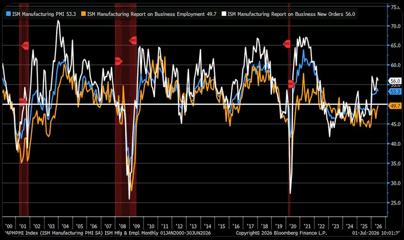
Employment is the recovery’s last unconvinced witness — the line that still won’t sign. Every deep manufacturing contraction on this chart was buried inside a recession: 2001, 2008-09, 2020, each troughed under a red bar. The 2023-2025 stretch broke that rule — 33 straight months of factory-payroll contraction, 41 of the last 42 since January 2023, the longest labor weakness here, and no recession bar covers it. Services and the consumer carried the load the factory floor dropped; this was a rolling sector recession the economy walked through, not into. Now the whole complex is inflecting, and the holdout is finally healing: Employment claws 1.1 points to 49.7, and the panel’s hiring-to-cutting comment ratio has near-reversed to 1.8:1 from 1:2 a year ago. The mechanism explains the lag. Firms met returning orders headcount-light — automation, productivity, post-2021 caution — while Prices at 73.0, propped by Section 232 tariffs and the Iran-war oil spike, froze the marginal hire; at 49.7, Employment still sits below the ~50.3 that maps to rising BLS payrolls, so mills shed workers, just slower. The forward risk is that the lead is already cresting: New Orders slipped -0.8 to 56.0, export orders back in contraction at 48.5. Anyone still short the goods cycle is positioned for a bottom that already passed.
Market Intelligence Brief (MIB) Ver. 18.40
For professional investors only. Not investment advice.
© 2026 RecessionALERT.com
MIB Daily: AI Is the Inflation the Fed Can’t Fight — JOLTS Beat #5 Lifts September Hike to 60%, USMCA Annual Track; Tech Most Exposed Thursday NFP
MARKET INTELLIGENCE BRIEF (MIB)
Tuesday, June 30, 2026
JOLTS beat for a fifth straight month at 7.594M, driving September rate-hike probability to 60%+ — same session S&P 500 closed Q2 +14.9% (best since 2020) and the Dow hit an all-time high. Cleveland Fed’s Hammack: AI infrastructure demand is a structural inflation force; rate hikes may be necessary. USMCA clean extension rejected — $1.5T North American trade enters annual review limbo. House Select probed MRK, LLY (-2.48%), PFE, ABBV, BMY over PLA hospital trials. SNDK +10.89% on $3,000 Bernstein PT.
TABLE OF CONTENTS
A. EXECUTIVE SUMMARY
B. MARKET DATA
C. HIGH-IMPACT STORIES (5)
D. MODERATE-IMPACT STORIES (6)
E. ECONOMY WATCH (6)
F. EARNINGS WATCH (0)
G. WHAT’S NEXT
H. CHART OF THE DAY
A. EXECUTIVE SUMMARY -> TOP
The S&P 500’s +14.9% Q2 — best since 2020 — and the Dow’s all-time high at 52,318 are the record-book result of a quarter-end relief rally that did not resolve the macro tension it inherited. The fifth consecutive JOLTS beat (7.594M vs. 7.3M) and Cleveland Fed President Hammack’s Sintra declaration that AI infrastructure demand is structural inflation drove September rate-hike probability from 20% to 60%+ on the same session — validating the AI/growth thesis while simultaneously threatening its valuation assumptions. Fund managers who underperformed now face benchmark pressure to add equity in Q3, but Technology (+39.24% Q2) — the most extended sector entering that quarter — is also most exposed to rate-hike repricing if Thursday’s NFP validates what JOLTS is already signaling. Six of 11 sectors red or flat is not breadth: it is the market pricing a narrowing growth story where only AI infrastructure capex and adjacent industrials clear the risk/reward bar.
• JOLTS May: fifth consecutive beat at 7.594M (vs. 7.3M consensus) — September rate-hike probability surged from ~20% to 60%+; July hike odds at 30%; 2-year Treasury yield +3.1 bps as rate futures repriced immediately
• Hammack (Sintra, Cleveland Fed): AI infrastructure demand is a “structural” inflation force — not tariff-driven, not transitory; explicitly declined to take a July hike off the table; Warsh speech Wednesday 9 AM ET is the next key event
• Q2 record close: S&P 500 +14.9% (best Q2 since 2020); Dow second consecutive ATH at 52,318 (+8.9% H1, best H1 since 2021); Nasdaq +21.4% Q2 — offset by Consumer Confidence miss (91.2 vs. 94.7) with “jobs hard to get” at a 5-year high
• USMCA: US refused clean extension — $1.5T North American trade relationship enters decade-long annual review track from 2027; MXN and CAD as real-time confidence gauges; autos (GM, F, STLA), agriculture most exposed
• Pharma national security probe: House Select Committee on China opened investigations into MRK, ABBV, PFE, LLY (‑2.48%), BMY over clinical trials at PLA-affiliated hospitals and Xinjiang; July 17 disclosure deadline
• SNDK +10.89% on Bernstein’s $3,000 PT raise (AI flash storage LTA structure re-rates NAND from commodity to recurring-revenue; +857% YTD); DLR ‑4.5% on $3.5B Northern Virginia data center equity dilution
1. AI Infrastructure: Bull Catalyst and Inflation Trap Simultaneously — The same AI capex supercycle that drove Technology +39.24% Q2 and SNDK +857% YTD is the structural inflation force Hammack identified at Sintra. Hyperscalers paying “almost any price” for physical infrastructure makes AI demand price-insensitive, non-transitory, and immune to tariff normalization — placing the Fed in a policy trap where tightening to control AI-driven inflation compresses the multiples of the AI equities themselves. The market cannot sustain both a permissive Fed and an AI bull market at current PCE levels.
2. Rate-Hike Risk Hiding Beneath the Record Quarter — JOLTS beat #5, Hammack’s structural inflation thesis, Consumer Confidence’s 5-year “jobs hard to get” high, and GDPNow’s slide to 2.5% from 4.3% constitute a stagflation data set: labor demand firm in AI/government sectors while worker perception deteriorates and consumer spending growth decelerates. The Warsh Fed’s no-dot-plot communications regime amplifies every data print into a maximum-movement event — Thursday’s NFP carries outsized volatility risk in both directions.
3. USMCA Annual Review Track Adds a New North American Supply Chain Risk Layer — The shift from a stable 16-year extension to annual review leverage creates deal-killer uncertainty for capital allocation decisions across US‑Canada‑Mexico supply chains. US automakers running just-in-time manufacturing across the border and agricultural exporters dependent on duty-free access cannot underwrite 5‑10 year investment decisions against a rolling renegotiation framework — a direct cost-of-capital headwind not yet priced into sector valuations.
B. MARKET DATA -> TOP
US-Iran ceasefire durability — and a last-day AI/semis surge — lifted the S&P 500 to close Q2 as its best quarter since 2020, with the Dow touching an all-time high of 52,317. The rally was selective rather than broad: Technology (+2.67%) and Industrials (+1.81%) surged while only five of eleven sectors closed green. Rate-sensitive Real Estate (-1.92%), Utilities (-1.36%), and Consumer Defensive (-1.46%) were the session’s biggest losers as the 10-Year yield rose +4.5 bps — a rising-rate headwind hiding beneath the headline optimism. For a PM: a quarter-end risk-on tone with unresolved bond non-participation; the terminal rate debate is still open.
CLOSING PRICES – Tuesday, June 30, 2026:
MAJOR INDICES
Nasdaq led on an AI/semis surge (+1.69%) as Dow industrials hit an all-time high — but transports fell -0.80%, opening a 1.06% DJIA/DJTA same-day spread that stops short of formal Dow Theory non-confirmation yet flags transport underperformance against the industrial advance. Key breadth signal: Russell 2000 extends its 9th consecutive session outpacing the S&P 500 — small-caps up +1.98% vs large-caps down -0.74% over 10 sessions — an entrenched broad-participation read. Five of 11 sectors green confirms the advance was concentrated in tech and industrials, not a market-wide sweep.
| Index | Close | Change | %Move | Why It Moved |
|---|---|---|---|---|
| S&P 500 | 7,498.79 | +58.36 | +0.78% | Iran ceasefire durability + AI/semis rebound wrapped S&P’s best Q2 since 2020; broad index gains partially offset by rate-sensitive sector declines |
| Dow Jones | 52,317.81 | +135.07 | +0.26% | All-time high close; blue-chip advance (+0.26%) lagged tech-heavy indices as Dow composition skews less toward high-beta semiconductor names |
| DJ Transportation | 21,749.0 | -176.00 | -0.80% | Bucked broader advance; quarter-end rotation into tech/semis drew capital from transport names; DJTA 2.7% below its 10-session high while Dow industrials hit new ATH |
| Nasdaq 100 | 30,276.35 | +501.60 | +1.69% | AI/semis surge led — AMD +7.68%, KLAC +8.38%, MRVL +7.25%, SNDK +10.89%; largest index percentage gainer on the session |
| Russell 2000 | 3,026.05 | +15.63 | +0.52% | Small-cap participation on domestic risk-on tone; 9th consecutive session outperforming S&P 500 over rolling 10-session window (+1.98% vs -0.74%) |
| NYSE Composite | 23,834.23 | +31.52 | +0.13% | Broad advance tempered by rate-sensitive sector selling; composite’s modest gain reflects the split between growth leaders and real estate/utilities declines |
VOLATILITY & TREASURIES
VIX slid -6.80% as Iran ceasefire anxiety unwound — but bond markets refused to confirm: 10Y yields rose +4.5 bps to 4.47% and 2Y yields added +3.1 bps on the same day equities rallied. That VIX-down/yields-up combination signals persistent inflation and rate-path anxiety, not risk-on consensus; in a genuine growth rally, bonds catch a bid alongside equities. The DXY barely moved (+0.07%), leaving the message unambiguous: the terminal rate debate is unresolved at quarter-end.
| Instrument | Level | Change | Why It Moved |
|---|---|---|---|
| VIX | 16.45 | -1.20 (-6.80%) | Iran ceasefire holding reduced tail-risk premium; VIX approaching its 10-session low as quarter-end fear unwinds |
| 10-Year Treasury Yield | 4.467% | +4.5 bps | Sticky inflation expectations + quarter-end duration selling; bond market declining to confirm equity rally — inflation narrative unresolved by ceasefire |
| 2-Year Treasury Yield | 4.170% | +3.1 bps | Near-term rate path uncertainty; Fed-on-hold narrative intact; 10Y-2Y spread at 29.7 bps (curve steepening modestly from 28.3 bps prior) |
| US Dollar Index (DXY) | 101.17 | +0.07 (+0.07%) | Effectively flat; quarter-end rebalancing flows offset Iran ceasefire pressure; dollar holding mid-range despite equity risk-on tone |
COMMODITIES
All four precious metals and copper posted modest gains — a quiet, corroborating session with no dramatic cross-commodity divergence. Gold holding near $4,026 signals residual safe-haven demand persisting despite ceasefire relief; the metal’s floor is higher than its pre-escalation baseline, anchored by sticky inflation and rate uncertainty. Bitcoin’s -2.82% decline against a risk-on equity tape is the standout: crypto-specific selling decoupled from the broader risk revival, suggesting profit-taking or on-chain dynamics rather than a macro sentiment signal.
| Asset | Price | Change | %Move | Why It Moved |
|---|---|---|---|---|
| Gold | $4,025.95/oz | +$4.30 | +0.11% | Modest safe-haven demand persists; gold holding above $4,000 despite ceasefire relief — floor anchored by sticky inflation and unresolved rate uncertainty |
| Silver | $59.175/oz | +$0.132 | +0.22% | Tracking gold higher; industrial demand component supported by AI/electrification tailwinds |
| Copper | $6.2535/lb | +$0.0068 | +0.11% | Industrial metals holding; China demand outlook stable; AI/electrification build-out supporting medium-term copper demand |
| Platinum | $1,561.75/oz | +$2.70 | +0.17% | Modest gain tracking precious metals complex; automotive and industrial demand steady |
| Bitcoin | $58,637 | -$1,704 | -2.82% | Declined against risk-on equity tape — crypto-specific selling decoupled from broader risk sentiment; profit-taking at prior resistance levels |
ENERGY
WTI and Brent effectively flat (-0.21% and +0.01%) — Iran sanctions relief has been fully absorbed over the past 18 sessions as WTI fell from $84 to $70 since June 12; the geopolitical risk premium is spent. Oil moving sideways alongside a +0.78% equity gain is a growth-neutral read: no new demand acceleration or supply catalyst. Dutch TTF +1.93% while Henry Hub barely moved (-0.15%) — European gas market recovering on its own storage and supply dynamics, fully diverging from US gas fundamentals.
| Asset | Price | Change | %Move | Why It Moved |
|---|---|---|---|---|
| Crude Oil (WTI) | $69.92/bbl | -$0.15 | -0.21% | Essentially flat; Iran sanctions relief fully absorbed (WTI fell ~$14 since June 12); OPEC+ production outlook now the primary price driver |
| Crude Oil (Brent) | $73.40/bbl | +$0.01 | +0.01% | Fractionally positive; WTI/Brent spread at $3.48 — narrow spread signals global rather than regional supply dynamics; no new disruption premium building |
| Natural Gas (Henry Hub) | $3.255/MMBtu | -$0.005 | -0.15% | Effectively flat; US natural gas fundamentals unchanged; summer demand tracking seasonal norms |
| Natural Gas (Dutch TTF) | $14.54/MMBtu | +$0.28 | +1.93% | European gas market recovering independently; UK/European storage refill demand and LNG supply tightness diverging from US fundamentals; TTF/Henry Hub spread widening |
S&P 500 SECTORS
Technology (+2.67%) rebounds from a -1.22% monthly slump but remains the quarter’s structural leader (+39.24% 3M) — today’s move is mean-reversion amplified by the AI catalyst, not a new trend break. Rate-sensitive sectors took the hardest hits: Real Estate (-1.92%), Utilities (-1.36%), and Consumer Defensive (-1.46%) sold off simultaneously as 10Y yields rose +4.5 bps — the rate pressure hiding beneath the headline gains. Healthcare (-0.96%) consolidates after leading the week (+4.63%) and month (+6.61%); the pullback is tactical, not structural, given its 3M and 12M persistence.
| Sector | 1-Day | 1-Week | 1-Month | 3-Month | 6-Month | YTD | 12-Month |
|---|---|---|---|---|---|---|---|
| Technology | +2.67% | +3.14% | -1.22% | +39.24% | +21.80% | +23.62% | +39.94% |
| Industrials | +1.81% | +4.35% | +5.90% | +19.98% | +19.78% | +21.83% | +30.37% |
| Basic Materials | +0.75% | -1.03% | -7.30% | +1.56% | +5.44% | +8.92% | +34.64% |
| Consumer Cyclical | +0.12% | +3.02% | -4.46% | +9.89% | -6.37% | -4.29% | +3.83% |
| Financial | +0.02% | -0.20% | +4.36% | +13.96% | +0.35% | +1.82% | +11.69% |
| Communication Services | -0.07% | +1.08% | -7.42% | +12.19% | -1.30% | -0.92% | +17.77% |
| Energy | -0.48% | -2.73% | -6.02% | -13.52% | +19.70% | +18.49% | +24.63% |
| Healthcare | -0.96% | +4.63% | +6.61% | +11.72% | +2.98% | +4.19% | +20.62% |
| Utilities | -1.36% | +0.51% | +1.31% | -0.84% | +5.75% | +6.30% | +13.74% |
| Consumer Defensive | -1.46% | -1.26% | +0.56% | +0.28% | +5.54% | +6.27% | +4.36% |
| Real Estate | -1.92% | -0.62% | +1.15% | +10.21% | +8.19% | +8.98% | +8.11% |
TOP MEGA-CAP MOVERS:
GAINERS
| Company | Ticker | Close | Change | Why It Moved |
|---|---|---|---|---|
| Sandisk Corp | SNDK | $2,273.73 | +10.89% | Bernstein raised price target to $3,000 from $1,700 (Outperform); 2026’s best S&P 500 performer (+857% YTD); AI-driven flash storage demand narrative intact; parent WDC fell as capital rotated to the spinoff |
| KLA Corp | KLAC | $301.71 | +8.38% | Semiconductor equipment surge on AI/tech rebound; Iran ceasefire removed global-supply-chain risk overhang; semis equipment names disproportionately benefited from sector re-rating |
| Advanced Micro Devices | AMD | $580.91 | +7.68% | AI chip rebound; semiconductor sector led the quarter-end recovery; concerns that AI stocks had gone too high partially unwound on solid demand signals |
| Marvell Technology | MRVL | $297.89 | +7.25% | AI data center networking and custom chip demand acceleration; broader semis complex re-rating on Iran ceasefire + AI spending narrative normalization |
| GE Vernova | GEV | $1,174.86 | +6.56% | AI data center power infrastructure demand driving electricity grid equipment orders; Industrials led the market (+1.81%) and GEV significantly outpaced the sector |
DECLINERS
| Company | Ticker | Close | Change | Why It Moved |
|---|---|---|---|---|
| Netflix | NFLX | $71.40 | -3.23% | Sustained downtrend continues: META expanding Instagram for TV to Samsung smart TVs + FOXA’s $22B Roku acquisition reshaping streaming landscape; Reed Hastings departure weighing; stock down ~40% from June 2025 ATH |
| Eli Lilly | LLY | $1,199.43 | -2.48% | Healthcare sector rotation/profit-taking after sector led the week (+4.63%) and month (+6.61%); weight-loss drug competition concerns persist; broader defensive selling on risk-on rotation |
| Western Digital | WDC | $638.72 | -2.02% | Spinoff Sandisk (SNDK) surged +10.89% on Bernstein analyst upgrade; capital rotating from parent WDC into the higher-momentum spinoff |
| Citigroup | C | $139.96 | -1.78% | Rising yield headwind (10Y +4.5 bps); quarter-end rebalancing out of Financials; bank margin compression concerns as curve steepens modestly |
| Johnson & Johnson | JNJ | $253.97 | -1.76% | Healthcare sector selling; defensive names underperformed on broad risk-on rotation; JNJ’s pharmaceutical pipeline concerns and litigation overhang continue to weigh |
C. HIGH-IMPACT STORIES -> TOP
BEARISH
1. JOLTS May Beats for Fifth Straight Month at 7.594M — September Rate Hike Probability Surges to 60%+
The core facts:May JOLTS job openings came in at 7.594 million versus the 7.30 million consensus — the fifth consecutive beat and the highest reading since May 2024 — reaffirming that US labor demand remains structurally firm despite five months of “low-hire, low-fire” payroll data. Markets repriced the Fed’s rate path immediately upon release: September rate hike probability surged from approximately 20% to 60%+, and July hike odds moved to approximately 30%, both per CME FedWatch. The 2-year Treasury yield rose sharply as rate futures absorbed the stronger-than-expected demand signal, compressing near-term rate-cut pricing entirely from the forward curve.
Why it matters:The JOLTS beat creates a direct contradiction at the heart of the Fed’s dual mandate: job openings at a two-year high confirm labor demand resilience that, at 4.1% headline PCE and 3.4% Core PCE, leaves the Fed with no easing room. Five consecutive above-consensus JOLTS prints signal that the structural labor tightness — driven partly by Hammack’s “insatiable” AI infrastructure capex demand — is not a seasonal anomaly but a durable feature of the post-tariff, AI-driven economy. For rate-sensitive assets, the repricing is asymmetric: the 60% September hike probability is not fully priced into long-duration bonds or high-multiple tech equities, creating residual downside risk for both asset classes if Thursday’s NFP confirms the labor market’s resilience. The Warsh Fed’s deliberate communication restraint — no dot-plot, shorter statements — amplifies the volatility: with no forward guidance to anchor expectations, each data print creates maximum market movement rather than incremental updating against a stated path. Today’s JOLTS print, combined with Hammack’s explicit rate hike warning from Sintra (see Story 2), represents the strongest single-day endorsement of a 2026 tightening scenario since the hiking cycle discussion began.
What to watch:Thursday July 2 NFP at 8:30 AM ET versus Pantheon’s 75K forecast — a strong print above 150K would push September hike probability to near-certainty; a 75K miss would sharply deflate hike odds despite today’s JOLTS strength. Fed Chair Warsh’s speech Wednesday July 1 at 9:00 AM ET for whether he validates or pushes back on the hike narrative before NFP.
BEARISH
2. Cleveland Fed’s Hammack: AI Infrastructure Is a Structural Inflation Driver — Rate Hike May Be Necessary
The core facts:Cleveland Federal Reserve President Beth Hammack, speaking Tuesday from the ECB’s Sintra forum in Portugal, stated explicitly that AI infrastructure demand is fueling inflation and that rate increases may be needed if elevated prices persist. Hammack cited an Ohio-based manufacturer of electric switching equipment for data centers, noting that hyperscalers “will pay almost any price” for AI infrastructure inputs — framing AI capex as a demand-pull inflation driver rather than a cyclical or tariff-driven phenomenon. “If inflation continues to persist at these elevated levels and I don’t see any restraint from policy, we may need to raise rates,” she said. Hammack is a voting FOMC member in 2026 — she dissented at the June FOMC meeting — and was speaking on the same day as the fifth consecutive JOLTS beat.
Why it matters:Hammack’s AI-inflation framing is analytically distinct from the standard tariff-passthrough narrative that has dominated the inflation discourse since early 2026. She is identifying AI infrastructure capex as a structural demand-pull force — one that is not transitory, not tariff-dependent, and not addressable through supply-chain normalization. This is a more durable and harder-to-dismiss inflation thesis than any trade-war framing: if hyperscalers are price-insensitive buyers of physical infrastructure inputs (power, data center electrical equipment, fiber, cooling), then the Fed cannot rely on goods disinflation to offset service-sector stickiness. Hammack’s position directly contradicts Chair Warsh’s baseline view that AI productivity gains will prove disinflationary — creating an explicit intra-FOMC policy disagreement now visible in real-time at a globally watched forum. The market’s immediate read: her hawkish signal, combined with today’s JOLTS beat, collectively increases the probability that the June 2026 FOMC was not the rate peak. For long-duration Treasuries, utilities, REITs, and high-multiple technology names, a structural AI-inflation thesis — if it gains traction with additional FOMC members — is a persistent valuation headwind that rate-cut pricing cannot resolve.
What to watch:Fed Chair Warsh speech Wednesday July 1 — specifically whether he addresses the AI-inflation framing and affirms his disinflation baseline or signals openness to Hammack’s structural thesis; any additional FOMC voter commentary in the pre-NFP window as the rate hike probability solidifies.
BULLISH
3. S&P 500 Caps Best Quarter Since 2020 (+14.9%); Dow Closes at Second Consecutive Record 52,319 — Best H1 Since 2021
The core facts:US equity markets closed June 30 with historic quarterly and half-year milestones. The Dow Jones Industrial Average set a second consecutive all-time high close at 52,319.20 (+136.46, +0.3%), locking in the best first half since 2021 (+8.9% H1). The S&P 500 advanced +0.79% to approximately 7,449–7,499, completing Q2 2026 with a gain of +14.9% — the best quarter since Q3 2020 during the COVID recovery. The Nasdaq Composite surged +1.52% to 26,213.72, finishing Q2 +21.4%. Technology led all 11 S&P 500 sectors at +2.67% for the session and +39.24% over the quarter. The Russell 2000 gained +0.46% to 3,024.37, crossing a new milestone as the quarter-end rally broadened beyond mega-cap names. The primary catalysts for the Q2 record run: the June 29 Supreme Court ruling preserving Fed independence (removing FOMC composition risk), Alphabet’s Dow inclusion creating forced passive buying, AI/semiconductor sector re-rating as the AI capex supercycle thesis survived the OpenAI IPO delay narrative, and the US-Iran ceasefire removing the energy shock that had pressured risk assets since late 2025.
Why it matters:Quarter-end performance benchmarks matter structurally: mutual funds and institutional managers who missed the Q2 rally face pressure to increase equity exposure in Q3 to track benchmarks, creating a systematic forced-buy dynamic that supports prices even if macroeconomic data — JOLTS beats, Hammack hike warnings, bimodal rate markets — complicates the forward picture. The S&P 500’s +14.9% Q2 is doubly significant because it follows a Q1 that was more modest — meaning the H1 2026 total return has materially outperformed the “stagflation” consensus that emerged in Q1 on tariff anxiety and Iran war risk. For portfolio managers rebalancing into Q3, the tactical question is whether to ride the momentum or reduce equities to lock in the historic quarterly gain: the Warsh Fed’s deliberate ambiguity — no dot-plot, shorter statements — creates maximum uncertainty about the Q3 macro backdrop, which historically argues for profit-taking after a 15% quarter. The technology sector’s +39.24% quarterly gain positions it as the most extended and most rate-sensitive sector entering Q3 — any additional rate hike pricing will disproportionately pressure tech valuations.
What to watch:July inflows data and fund positioning reports for whether institutional buyers accelerate equity allocation after the record Q2, or lock in gains; Thursday July 2 NFP as the first Q3 data test of whether the macro backdrop supports the current valuation multiple.
UNCERTAIN
4. US Refuses Clean USMCA Extension at Mandated 2026 Review — Annual Review Track Triggered, North American Trade Uncertainty Deepens
The core facts:At the USMCA’s mandated July 1, 2026 joint review, the United States signaled it will not grant a clean extension of the United States-Mexico-Canada Agreement. US Trade Representative Jamieson Greer confirmed he was not prepared to recommend clean renewal, and President Trump has publicly stated he is “not looking to renew” the deal as structured. Under the USMCA’s sunset clause, a refusal by any one party to agree to an extension triggers a decade-long annual review track beginning in 2027 — the agreement does not terminate immediately but enters a rolling renegotiation cycle that can extend to 2036. The Trump administration’s preferred outcome is a bilateral restructuring with annual reviews, using the USMCA review as leverage to extract concessions from Canada and Mexico on trade disputes, migration, drug trafficking, and continental defense matters. A “clean extension” — one that preserves the existing text for an additional 16 years — is now off the table.
Why it matters:USMCA governs approximately $1.5 trillion in annual trade between the US, Canada, and Mexico — the world’s largest tripartite trade relationship. The shift from a stable 16-year extension framework to an annual review track introduces a new category of political risk: North American supply chain stability is now subject to year-over-year renegotiation leverage, meaning any geopolitical friction (auto content disputes, Canadian dairy, Mexican energy nationalism) can be weaponized at an annual review. For US-listed companies with deeply integrated North American supply chains — autos (GM, Ford, Stellantis), agriculture, semiconductor manufacturing inputs, and energy — the inability to make 5-10 year capital allocation decisions against a stable USMCA framework increases their cost of capital. The most immediate sector exposures: US automakers whose plants are split across US-Mexico supply chains (critical for just-in-time manufacturing), US agricultural exporters dependent on duty-free access to Canada and Mexico, and the Canadian dollar and Mexican peso as the real-time market sentiment gauges. The base case — a “painful extension” with renegotiation stretching into late 2026 — is not a benign outcome: a prolonged negotiation gap creates deal-killer uncertainty for M&A and capital investment in all three economies.
What to watch:Canada and Mexico’s formal response to the US non-extension signal — whether they respond as a trilateral bloc or seek bilateral tracks separately; Mexican peso (MXN) and Canadian dollar (CAD) as real-time confidence gauges; any Trump executive action using the review as leverage for non-trade concessions.
UNCERTAIN
5. US-Iran Doha Technical Talks Proceed Without Direct Contact; WTI Holds Near $70 as API Reports 6.072M-Barrel Crude Draw
The core facts:The first Doha diplomatic engagement following the June 24 ceasefire declaration proceeded Tuesday with US Special Envoy Steve Witkoff and Jared Kushner meeting Qatari Prime Minister Sheikh Mohammed bin Abdulrahman as mediators. Iranian delegations participated separately — the US and Iran are not meeting directly — with Pakistan and Qatar serving as interlocutors. The structure mirrors Iran’s stated position that its technical experts will not negotiate directly with US counterparts, limiting the talks’ near-term scope. Concurrently, the American Petroleum Institute reported a 6.072 million barrel crude draw for the week ended June 27 — more than 50% above the 4.1 million barrel consensus and dramatically above the prior week’s -0.765 million barrel draw — the largest weekly crude inventory decline since April. WTI crude held near $70 per barrel; the benchmark is down approximately 19% month-to-date and 24% quarter-to-date from the war-premium highs. Gold fell alongside oil, closing Q2 at approximately $4,000 — its worst quarterly performance in 13 years — as Iran war risk premia unwound throughout the quarter.
Why it matters:The indirect negotiation structure in Doha confirms the analytical point from yesterday’s report: Iran’s refusal to allow direct technical talks limits the pace of ceasefire formalization. The risk scenario is not a ceasefire collapse but a prolonged limbo — neither a full normalization that removes all risk premium nor an active conflict that reinstates it. Oil markets are reading the ceasefire as durable at current WTI levels (~$70), but the 6.072M API draw introduces a counternarrative: US crude inventory is being drawn at a pace that suggests either front-running of Iranian crude re-entry (importers buying ahead of anticipated supply glut) or demand recovery stronger than the bearish price tape implies. JPMorgan and Citi’s ~4M bbl/day oversupply thesis (from yesterday’s report) remains the structural medium-term bear case, but the API draw signal creates near-term technical support. For US energy equities, the dual signal — ceasefire holding but talks moving slowly, inventory drawing bullishly but structural oversupply looms — creates a range-bound sector with no obvious directional catalyst until the Doha talks produce concrete outcomes on Strait of Hormuz passage guarantees and Iranian crude re-entry timelines.
What to watch:Wednesday EIA weekly petroleum status report to confirm or contradict the API 6.072M draw; whether Doha talks advance to direct US-Iran technical contact by Thursday; WTI’s hold above $68 as the ceasefire durability price floor.
D. MODERATE-IMPACT STORIES -> TOP
BEARISH
6. CB Consumer Confidence Misses at 91.2 — “Jobs Hard to Get” Hits Five-Year High, Compressing Discretionary Spending Outlook
The core facts:The Conference Board Consumer Confidence Index for June came in at 91.2, missing the 94.7 consensus estimate. The “Jobs Hard to Get” subcomponent rose to 22.5% — the highest reading since January 2021 — signaling that US consumers increasingly perceive labor market access as more difficult even as JOLTS job openings remain at a two-year high. The divergence between employer demand (strong openings data) and worker perception (elevated “jobs hard to get”) signals a structural mismatch rather than broad-based labor market tightness. Released on the same day as the JOLTS beat, the consumer confidence miss compounds the bifurcated macro picture: demand for labor is firm, but workers are not experiencing that demand as accessible opportunity.
Why it matters:Consumer confidence at 91.2 with “jobs hard to get” at a five-year high is a 2-3 month leading indicator for the unemployment rate — historical patterns suggest elevated “hard to get” readings precede unemployment rate increases. For consumer discretionary equities and retail, the miss argues for a more cautious Q3 consumer spending trajectory: households perceiving difficulty finding work tend to increase precautionary savings and reduce discretionary outlays, compressing margins for mid-to-high discretionary retailers. The simultaneous JOLTS-strong / confidence-weak combination suggests that AI-driven data center construction and government infrastructure are absorbing labor demand, while traditional consumer-facing service sector hiring is decelerating — a sector-bifurcated labor market that suppresses broad wage growth despite aggregate openings strength.
What to watch:Thursday July 2 NFP unemployment rate — whether the “jobs hard to get” signal begins to appear in the headline rate; next retail sales print for confirmation of the consumer spending deceleration thesis.
BEARISH
7. Chicago PMI Decelerates Sharply to 56.7 — Largest Monthly Drop Since Late 2025, Raises Stakes for Wednesday’s ISM Manufacturing
The core facts:The Chicago Business Barometer (Chicago PMI) for June fell to 56.7 from 62.7 in May, against expectations of 58.1 — the largest single-month deceleration since late 2025. The reading remains in expansion territory (above 50) but the magnitude of the decline interrupts the manufacturing re-acceleration narrative that had built over Q2 as tariff front-running drove order backlogs. The Dallas Fed’s June Business Activity Index was 0.0 (reported yesterday) — stalling at neutral from +0.4 in May — reinforcing the Chicago signal. ISM Manufacturing PMI for Wednesday July 1 carries a consensus of 54.0 (matching May’s reading); ISM Prices Paid is expected to ease from 82.1 to approximately 79.
Why it matters:Chicago PMI’s 6-point deceleration raises the probability that Wednesday’s ISM Manufacturing prints below 54.0 — an outcome that would confirm a manufacturing plateau rather than acceleration, limiting industrials and materials sector re-rating into Q3. The more consequential sub-index is ISM Prices Paid: an easing from 82.1 to 79 would be the first meaningful input-cost moderation in months — reducing the Fed’s goods-sector inflation anxiety and incrementally supporting a September cut scenario. But if Prices Paid remains elevated (82+), it would reinforce Hammack’s AI-infrastructure supply-demand tightness thesis and strengthen hike arguments. The Chicago deceleration also signals potential tariff front-running demand exhaustion: if businesses pulled forward Q2 orders to beat tariff deadlines, Q3 ordering rates could slow further, extending the manufacturing softness into a period when the Fed cannot offset with accommodation.
What to watch:Wednesday July 1 ISM Manufacturing PMI — a print below 52 would signal a genuine manufacturing deceleration; ISM Prices Paid specifically, with above 82 being the threshold that strengthens the September hike case.
UNCERTAIN
8. Digital Realty Acquires Blackstone’s 64% Stake in Three Northern Virginia Data Centers for $3.5B — DLR -4.5% on Equity Dilution
The core facts:Digital Realty Trust (DLR) closed its acquisition of Blackstone’s blended 64% equity interest in three fully leased hyperscale data centers in Northern Virginia, paying $3.5 billion in total consideration ($1.2 billion cash, $2.3 billion in DLR shares). The assets — located in Manassas (two centers) and Sterling (one on the Digital Dulles campus) — collectively hold 288 megawatts of total IT capacity and are 100% leased to three distinct investment-grade hyperscale customers. The gross asset value is $7.8 billion, implying a cap rate of approximately 6.5% upon stabilization. DLR fell -4.5% on the equity issuance, as the $2.3 billion in share consideration dilutes existing shareholders. For Blackstone, the sale at a $7.8 billion portfolio valuation represents a profitable exit from data center assets it has held through the AI demand surge.
Why it matters:The transaction is a data point in the ongoing price discovery process for hyperscale data center assets — and the 6.5% cap rate on fully-leased Northern Virginia assets is the market’s current clearing price for prime AI infrastructure real estate. Northern Virginia is the world’s largest data center market, and a 100%-leased, investment-grade-tenant portfolio transacting at $27M per megawatt ($7.8B ÷ 288 MW) sets a benchmark for comparable assets. DLR’s -4.5% reaction signals that markets view the equity dilution as an expensive growth path — investors are discounting the strategic value of the expansion against the share count increase. The deal arrives on the same day Realty Income announced a separate data center joint venture seeded with assets valued over $6 billion, confirming a structural shift in REIT capital allocation toward hyperscale AI infrastructure. The simultaneous DLR and Realty Income announcements on June 30 reflect the AI data center buildout as now a defining theme for real estate capital markets, compressing traditional retail and office REIT strategies in favor of compute infrastructure.
What to watch:DLR’s post-close equity stabilization as index funds absorb the dilution; cap rate trajectory for comparable Northern Virginia hyperscale assets as the next benchmark; DLR Q3 earnings for color on hyperscale customer demand and lease renewal pricing.
BEARISH
9. House Select Committee on China Opens National Security Investigation Into Merck, AbbVie, Pfizer, Eli Lilly, BMS Over Clinical Trials at Chinese Military Hospitals
The core facts:The House Select Committee on the Chinese Communist Party, chaired by Representative John Moolenaar (R-MI), launched national security investigations into five of the largest US pharmaceutical companies — Merck, AbbVie, Pfizer, Eli Lilly, and Bristol Myers Squibb — over clinical trials conducted at Chinese military hospitals and in Xinjiang. The committee’s letters allege that Merck sponsored or collaborated in 224 clinical studies in China since 2005, including 40 at PLA-affiliated medical centers and at least 31 in Xinjiang. AbbVie conducted more than 100 clinical studies in China, including 16 at military centers and 17 in Xinjiang. Drugmakers have until July 17 to provide detailed due diligence, data protection processes, and site standards for their Chinese trial locations. The committee’s letters state there is “no evidence of illegal activity” but that conducting trials at PLA hospitals “exposes American companies to ethical and security risks” of IP transfer to the Chinese military.
Why it matters:The investigation targets five companies that collectively represent a significant share of the S&P 500 Healthcare sector, creating a regulatory overhang that could constrain their China clinical development strategies. For the broader pharma sector, the probe arrives at an already fraught moment: the July 31 implementation date for 100% tariffs on branded pharmaceutical imports means pharma equities are simultaneously absorbing tariff risk, pricing pressure narratives, and now a national security compliance inquiry. The China clinical trial investigation is particularly sensitive because it implicates the R&D pipeline — clinical data gathered at PLA-affiliated hospitals could face FDA review challenges if the committee’s concerns lead to regulatory action on trial integrity. For investors, the July 17 disclosure deadline is the first forcing function: companies whose responses reveal extensive PLA hospital exposure could face additional scrutiny, while companies that can demonstrate clean site protocols may differentiate. The investigation also reflects the bipartisan intensification of the China decoupling imperative across healthcare supply chains — following previous action on API manufacturing (active pharmaceutical ingredients) sourced from China, the probe now reaches clinical development itself.
What to watch:July 17 congressional disclosure deadline and whether any company’s response triggers follow-on regulatory or FDA action; FDA’s own position on trial data integrity from PLA-affiliated sites as the regulatory enforcement risk; sector reaction if additional pharma names beyond the initial five are identified.
BEARISH
10. Gold Ends Worst Quarter in 13 Years Near $4,000 — Hawkish Fed Repricing and Iran Ceasefire Unwind Safe-Haven Bid Accumulated Since January
The core facts:Gold closed Q2 2026 holding near $4,000 per ounce after falling approximately 11% for the quarter — its worst quarterly performance since Q3 2013, when the first taper tantrum drove a comparable precious metals rout. The quarter’s decline reverses a portion of gold’s extraordinary Q1 surge to a record high near $5,600 per ounce in January 2026, driven by Iran war escalation. The primary drivers of Q2’s decline: the US-Iran ceasefire unwinding the geopolitical risk premium accumulated during the conflict, the Fed’s hawkish pivot under Chair Warsh (nine FOMC members projecting at least one 2026 hike), rising real yields making the opportunity cost of holding non-yielding gold prohibitive at current 4%+ money market rates, and a stronger US dollar driven by the hawkish rate repricing. Gold ETF outflows indicate institutional allocators rotated out of precious metals toward risk assets during Q2, consistent with the equity markets’ best quarter since 2020.
Why it matters:Gold’s worst-quarter-in-13-years framing carries two portfolio-management implications. First, it is a retrospective confirmation of the Q2 risk appetite shift: money that flowed into gold during the Iran war hysteria has rotated back into equities, strengthening the Q2 equity rally’s duration but also leaving gold exposed if macro conditions shift. Second, it is a forward-looking signal about the Fed’s credibility at current PCE levels: gold at $4,000 despite 4.1% headline inflation indicates markets believe the Warsh Fed will tighten sufficiently to restore price stability — gold would be closer to $5,000+ if markets expected the Fed to fall behind the curve. The $4,000 support level is technically and psychologically significant: a break below it would signal intensified expectations of Fed tightening that could also pressure equities; a recovery above $4,200 would suggest inflation expectations are re-anchoring higher despite today’s hawkish repricing. For portfolio construction, gold’s 11% Q2 decline compresses the traditional equity-gold diversification benefit — if both assets are now positively correlated (equities rally as gold falls on risk-on flows), alternative diversifiers (TIPs, commodities) become more relevant in Q3 allocations.
What to watch:Gold’s technical support at $4,000 — a break below that level would be a signal of accelerating hawkish repricing; Thursday NFP: a weak print (≤75K) could reverse gold as rate-cut odds spike; ETF flow data over the next two weeks for whether institutional gold selling has run its course.
BULLISH
11. Sandisk (SNDK) +5.47% as Bernstein Raises Price Target to $3,000 — Memory LTA Structural Shift Anchors AI Storage Supercycle
The core facts:Bernstein analyst Mark Newman raised the Sandisk Corporation (SNDK) price target from $1,700 to $3,000, maintaining an Outperform rating, driving the stock up approximately 5.47% on June 30. The analyst cited a fundamental structural shift in how memory manufacturers are structuring long-term supply agreements (LTAs) with hyperscale customers: fixed or range-bound pricing, upfront financial commitments, and 3-5 year contract terms. At $3,000, Bernstein’s target implies approximately 50% additional upside from current prices despite SNDK already being the S&P 500’s best-performing stock year-to-date with an approximately 857% gain. The $3,000 target is derived from 11x Bernstein’s FY2028 EPS estimate or 14x the FY2026-2030 through-cycle average EPS. Sandisk’s parent lineage (spun from Western Digital) makes it the pure-play flash and NAND memory vehicle for the AI storage buildout.
Why it matters:The LTA pricing structure Bernstein identifies is the memory sector’s equivalent of the defense industry’s long-term contracts: it transforms NAND flash from a notoriously cyclical commodity into a recurring-revenue technology business with predictable cash flows. For investors, this re-rating thesis is durable rather than cyclical: if hyperscalers are committing to 3-5 year fixed-price memory supply agreements, Sandisk’s earnings volatility — historically the primary reason memory stocks trade at discounts to the broader semiconductor sector — is structurally compressed. The LTA development is also competitively significant: if Sandisk has locked in hyperscaler commitments at fixed pricing, rivals (Samsung, SK Hynix) face structurally reduced addressable markets for spot and contract NAND sales to the same customer set. Bernstein’s $3,000 target, using through-cycle EPS averaging, signals that the analyst believes the LTA structure eliminates the down-cycle risk that traditionally forces through-cycle EPS discounting — an unusually high-conviction call at an already-extreme trailing valuation. With WDC (parent company) falling -2.02% as capital rotates to the purer SNDK vehicle, the market is explicitly pricing the spinoff premium as a structural, not transitory, feature.
What to watch:Samsung and SK Hynix pricing behavior in response to SNDK’s LTA-driven demand lock-in; SNDK next quarterly results for confirmation that fixed-price LTA volumes are displacing spot contract mix; whether other memory names (MU, SK Hynix ADR) see comparable LTA adoption.
E. ECONOMY WATCH -> TOP
June 30’s data delivered a hawkish-growth paradox: JOLTS job openings posted a fifth consecutive beat (7.594M vs. 7.30M est.), endorsing Cleveland Fed President Hammack’s same-day warning that AI-fueled demand may necessitate rate hikes. Yet the consumer is fraying — confidence missed by 3.5 points (91.2 vs. 94.7 est.) with “jobs hard to get” at its highest since January 2021. The Chicago PMI decelerated sharply to 56.7 (prior 62.7), and GDPNow has slipped to 2.5% from a May peak of 4.3% as PCE growth is revised lower. Fed Chair Warsh’s July 1 speech and Thursday’s June payrolls (consensus 110K) are the week’s binary risk pivots.
JOLTS Job Openings Beat for Fifth Straight Month at 7.594M, Endorsing Fed Hike Bets (BLS, June 30, 2026)
What they’re saying:US job openings rose to 7.594 million in May, beating the 7.30M consensus by 294,000 — the fifth consecutive beat of estimates and the highest level in over two years. The prior reading held near the same level at 7.585M. Job quits rose to 3.065M (from 2.977M prior), indicating workers remain confident enough to leave jobs voluntarily — a signal of continued labor market health.
The context:The persistent strength in labor demand leaves the Fed with little cover to ease policy. Markets repriced rate hike odds higher immediately following the print, with futures placing roughly 30% probability on a July hike and over 60% on tightening by September. The JOLTS beat directly amplifies Hammack’s June 30 hawkish message and keeps upward pressure on 2-year Treasury yields heading into Thursday’s payrolls report — the week’s single most important macro data point.
What to watch:June Nonfarm Payrolls (Thursday, Jul 2, 8:30 AM ET; consensus 110K, Pantheon 75K); Fed Chair Warsh speech (Wednesday, Jul 1, 9:00 AM ET).
Consumer Confidence Falls Short at 91.2 — “Jobs Hard to Get” Hits Five-Year High (Conference Board, June 30, 2026)
What they’re saying:The Conference Board Consumer Confidence Index rose just 0.6 points to 91.2 in June — a 3.5-point miss vs. the 94.7 consensus — while the prior month (May) was revised down from 93.1 to 90.6. The share of consumers saying jobs are “hard to get” climbed to 22.5%, the highest reading since January 2021. Falling gas prices offered partial relief but were insufficient to lift overall sentiment.
The context:The sharp deterioration in the labor market assessment — released simultaneously with a JOLTS beat — underscores a growing divergence: employers are still posting jobs, but workers increasingly feel those openings aren’t accessible. Historically, rising “jobs hard to get” readings lead the unemployment rate higher by two to three months. This confidence miss introduces risk that the consumer spending tailwind supporting PCE through H1 2026 may fade into Q3, a development that would push GDPNow’s already-declining Q2 estimate lower.
What to watch:ADP Employment Change (Wednesday, Jul 1, 8:15 AM ET; consensus 113K); June Nonfarm Payrolls (Thursday, Jul 2, 8:30 AM ET); July Consumer Confidence (late July).
Cleveland Fed’s Hammack: AI-Driven Demand Could Force Rate Hikes — July Not Off the Table (Cleveland Federal Reserve, June 30, 2026)
What they’re saying:Cleveland Fed President Beth Hammack stated that “insatiable” demand for artificial intelligence infrastructure may be a persistent and structural source of inflation. She said: “If inflation continues to persist at these elevated levels and I don’t see any restraint from policy, we may need to raise rates to bring that policy restraint in and to bring inflation back down.” She did not commit to a July FOMC hike, but explicitly declined to take one off the table.
The context:Hammack’s hawkish framing is notable for two reasons: it identifies AI capital expenditure — not tariffs — as the primary inflation driver, and it positions the Fed as potentially needing to act rather than simply wait. Polymarket’s Fed hike probability ticked up to 55% (from 53% prior session) following today’s JOLTS and Hammack combination. While she is not a 2026 FOMC voter, her remarks add institutional weight to the hiking scenario and may foreshadow the tone of Fed Chair Warsh’s speech Wednesday morning — the most consequential forward guidance event of the week.
What to watch:Fed Chair Warsh speech (Wednesday, Jul 1, 9:00 AM ET) — watch for any explicit endorsement or pushback on the rate hike framing.
Chicago PMI Slips to 56.7 in June, Missing Consensus and Cooling Sharply from May’s Four-Year High (MNI Markets, June 30, 2026)
What they’re saying:The Chicago Business Barometer fell to 56.7 in June from 62.7 in May, missing the 58.1 consensus estimate. The index remains well above the 50 expansion/contraction threshold, indicating continued Midwest business activity growth, but the 6-point single-month drop is the largest deceleration since late 2025. Separately, the Dallas Fed Services Index recovered to 2.9 in June from -7.7 in May, offering a partial offset at the regional level.
The context:The May surge to a four-year high of 62.7 was likely inflated by tariff front-running — businesses pulling forward purchases before new import costs took effect. The June normalization confirms that dynamic is unwinding. With the ISM Manufacturing PMI (broader and more closely watched) due Wednesday at an expected 54.0, the Chicago print introduces downside risk to that reading. An ISM print below 50 would flip the national manufacturing signal to contraction and materially reset Q3 growth expectations.
What to watch:ISM Manufacturing PMI June (Wednesday, Jul 1, 10:00 AM ET; consensus 54.0, prior 54.0); ISM Manufacturing Prices Paid (consensus 79, prior 82.1).
Atlanta Fed GDPNow Q2 2026 Estimate Slips to 2.5% as Consumer Spending Nowcast Revised Lower (Federal Reserve Bank of Atlanta, June 25, 2026)
What they’re saying:The Atlanta Fed’s GDPNow model places Q2 2026 real GDP growth at 2.5% in its most recent update (June 25), down from 3.0% on June 17 and a peak of 4.3% in late May. The primary driver of the most recent downward revision was a reduction in the nowcast of Q2 real personal consumption expenditures (PCE) growth from 2.7% to 2.0%. The next GDPNow update is scheduled for Wednesday, July 1 — it will incorporate today’s JOLTS and confidence data.
The context:A 1.8-percentage-point decline from the May peak suggests the tariff-driven front-running in consumer and business spending has largely exhausted itself. The 2.5% tracking estimate still represents healthy above-trend growth, but the directional trend matters: if today’s Conference Board miss foreshadows continued PCE softness, Wednesday’s GDPNow update may push the Q2 estimate closer to 2.0%. That level would still avoid a contraction but would mark the weakest quarterly growth since Q1 2023 and further complicate the Fed’s stagflation calculus.
What to watch:GDPNow update (Wednesday, Jul 1) incorporating today’s releases; June Nonfarm Payrolls (Thursday, Jul 2, 8:30 AM ET) — last major Q2 labor market data point before the advance GDP estimate.
FHFA Home Prices Dip 0.1% in April; Case-Shiller Shows 11th Straight Month of Real-Term Decline (FHFA / S&P Global, June 30, 2026)
What they’re saying:The FHFA monthly house price index fell 0.1% MoM in April, against a +0.2% consensus and a revised +0.2% prior reading. Year-over-year gains moderated to +2.0%. The S&P Cotality Case-Shiller 20-City Composite rose 1.1% YoY (up from 0.9% prior), but with CPI running at approximately 3.8% in April, home values declined in real (inflation-adjusted) terms for an eleventh consecutive month. Regional divergence remains sharp — Mountain division -0.8% MoM; New England +1.0% MoM.
The context:Housing is caught in a persistent dual headwind: elevated mortgage rates (30-year at 6.49%) continue to suppress affordability-driven demand, while constrained inventory limits price relief for buyers. The eleven-month streak of real-term price declines erodes household wealth for existing homeowners via the “wealth effect” — a meaningful headwind for consumer spending. A reversal would require either a significant rate cut (not currently priced before late 2026/2027) or a supply shock. Wednesday’s MBA Mortgage Applications data will indicate whether any rate-driven demand activity is emerging.
What to watch:MBA Mortgage Applications (Wednesday, Jul 1, 7:00 AM ET); 30-Year Mortgage Rate (Jul 3 print, currently 6.49%).
F. EARNINGS WATCH -> TOP
YESTERDAY AFTER THE BELL (Markets Reacted Today)
No major earnings yesterday after the bell from companies with >$100B market cap.
TODAY BEFORE THE BELL (Markets Already Reacted)
No major earnings before the bell from companies with >$100B market cap.
TODAY AFTER THE BELL (Markets React Tomorrow)
No major earnings after the bell from companies with >$100B market cap. Nike (NKE, $60.79B market cap) reports AMC tonight — below the >$100B inclusion threshold.
WEEK AHEAD PREVIEW:
Q1 2026 earnings season is effectively complete at 89% of the S&P 500 reported, with blended EPS growth of +27.7% YoY — the strongest quarter since Q4 2021. The week of June 30 – July 3 marks the seasonal trough before Q2 2026 earnings season opens. No mega-cap companies (>$100B market cap) are scheduled to report through Friday July 3; the next wave of major reporters is expected in mid-July, beginning approximately July 11 when FactSet publishes its Q2 2026 season-opening Earnings Insight.
Q2 2026 earnings season begins mid-to-late July with the major financial sector reporters (JPMorgan, Goldman, Citigroup, Wells Fargo, BlackRock) typically among the first large-caps to report — watch for JPMorgan’s Q2 date announcement as the de facto season-open signal.
G. WHAT’S NEXT -> TOP
UPCOMING RELEASES:
| Date | Event | Why It Matters |
|---|---|---|
| Wed, Jul 1 | Fed Chair Warsh Speech (9:00 AM ET) | Most consequential forward guidance event of the week — markets watching for whether Warsh validates Hammack’s AI-inflation thesis and September hike framing, or reaffirms his disinflation baseline. Any explicit endorsement of rate-hike language would accelerate bond selling and widen the rate-sensitive sector selloff heading into NFP. |
| Wed, Jul 1 | ISM Manufacturing PMI Jun (exp. 54.0, prior 54.0) | Chicago PMI’s 6-point deceleration to 56.7 introduces downside risk to this print. A sub-50 ISM would signal national manufacturing contraction and materially reset Q3 growth expectations; a stable 54.0 confirms expansion continues despite front-running demand exhaustion. |
| Wed, Jul 1 | ISM Manufacturing Prices Paid Jun (exp. 79, prior 82.1) | The most Fed-sensitive ISM sub-index. An easing from 82.1 to 79 would be the first meaningful input-cost moderation in months, incrementally supporting a September cut scenario. A hold above 82 reinforces Hammack’s structural inflation thesis and strengthens the hike argument before Thursday’s payrolls. |
| Wed, Jul 1 | ADP Employment Change Jun (exp. 113K, prior 122K) | Private-sector payroll preview for Thursday’s NFP. A print below 100K would raise probability that the Pantheon 75K NFP scenario materializes; a beat above 130K would add to JOLTS-driven confidence in labor market resilience and extend the September hike narrative. |
| Wed, Jul 1 | Construction Spending MoM May (exp. +0.2%, prior +0.4%) | Tracks AI data center and infrastructure buildout alongside residential construction. A deceleration would signal capex front-running is unwinding; an upside surprise would corroborate Hammack’s AI capex demand thesis and support the Industrials sector’s +19.98% Q2 run. |
| Thu, Jul 2 | Nonfarm Payrolls Jun (exp. 110K, prior 172K; Pantheon: 75K) | The week’s single most important data point. A print above 150K would push September hike probability to near-certainty and trigger broad repricing of long-duration Treasuries and high-multiple tech equities. A Pantheon-scenario 75K miss would sharply deflate hike odds despite JOLTS strength, reversing Tuesday’s rate repricing. Note: Friday Jul 3 is the NYSE-observed Independence Day holiday — this is the week’s final trading day. |
| Thu, Jul 2 | Initial Jobless Claims Jun 27 (exp. 220K, prior 215K) | Real-time labor market health check released alongside NFP. A spike above 240K would signal early cracks in the labor market consistent with Consumer Confidence’s “jobs hard to get” reading; a stable sub-220K print would reinforce the JOLTS narrative of structural tightness. |
| Thu, Jul 2 | Unemployment Rate Jun (exp. 4.3%, prior 4.3%) | A tick up to 4.4%+ would begin to validate Consumer Confidence’s 5-year “hard to get” high as a leading indicator; a hold at 4.3% keeps the Fed’s dual mandate in tension — openings strong, headline stable — and leaves September ambiguous until ISM and PCE data arrive. |
| Thu, Jul 2 | Average Hourly Earnings MoM Jun (exp. +0.3%, prior +0.3%) | Wage growth stability is the Fed’s services-inflation anchor. A +0.4%+ reading would add a wage-push inflation signal on top of JOLTS and Hammack’s AI-demand thesis, meaningfully strengthening the September hike case. |
| Thu, Jul 2 | Average Hourly Earnings YoY Jun (exp. +3.5%, prior +3.4%) | Year-over-year wage acceleration to 3.5% with headline PCE at 4.1% still leaves real wages negative — a consumer spending headwind that reinforces the Conference Board confidence miss. Any upside surprise above 3.6% would compound the Fed’s inflation calculus. |
KEY QUESTIONS:
1. Will Warsh’s Wednesday speech validate Hammack’s AI-inflation thesis — or push back on the rate-hike framing — before Thursday’s NFP data settles the September probability question for markets?
2. Does Thursday’s NFP confirm the labor market strength JOLTS is already signaling, locking in a September hike and triggering a repricing of Technology’s +39.24% Q2 valuation multiple before Q3 has fully begun?
3. Can the USMCA renegotiation be contained to a tolerable “painful extension” — or will the shift to annual review leverage trigger supply chain capital-allocation paralysis in autos and agriculture before a new framework is agreed?
H. CHART OF THE DAY -> TOP
Concentration has a fingerprint, and it just printed its widest reading in 35 years. The one-year correlation between the S&P 500 and its equal-weight twin has fallen to 79% — tied for the lowest since 1991 and roughly 4.25 standard deviations below the 96% norm, a tail so far out the chart’s axis can’t frame it. The index and the median stock it claims to hold have never moved less alike. The dot-com peak and the COVID melt-up punched correlation down too, but those were sharp, event-driven dislocations that snapped back within months once the catalyst passed. This is different in kind, not degree. It has ground near record lows for two to three years, and when it tried to heal — bouncing to ~92% — it failed, rolling straight back to a fresh low. That persistence is the tell: this is breadth narrowing rendered as a single number, cleaner than any advance-decline reading, the steady-state signature of a market where a few mega-caps carry the index while the median stock stalls. The implication cuts deepest for the $10T+ of household savings indexed to the cap-weighted S&P: they own breadth on paper and concentration in fact. The prior dips healed because the story ended. This one hasn’t started writing its ending.
Market Intelligence Brief (MIB) Ver. 18.40
For professional investors only. Not investment advice.
© 2026 RecessionALERT.com
MIB Daily: SCOTUS 5-4 and Iran Ease Spark Rally; Bond Non-Confirmation Warns — Overweight Semis, Fade Duration Into 75K NFP Thursday
MARKET INTELLIGENCE BRIEF (MIB)
Monday, June 29, 2026
The Supreme Court preserved Fed independence 5-4 (Lisa Cook stays) while overturning Humphrey’s Executor 6-3, sending the Nasdaq 100 to a 2.26% gain. NVIDIA’s $3.2B Corning AI deal drove GLW +15.7% and SOXX +3.76% as Alphabet debuted on the Dow, crossing 52,000. Iran’s ‘stand down’ unwound gold -1.60% but Doha talks Tuesday face structural friction. Pantheon projects Thursday’s NFP at 75K vs 172K in May — stagflation signal crystallizing. Strategy plans to sell $1.25B in Bitcoin, flipping BTC supply negative.
TABLE OF CONTENTS
A. EXECUTIVE SUMMARY
B. MARKET DATA
C. HIGH-IMPACT STORIES (5)
D. MODERATE-IMPACT STORIES (7)
E. ECONOMY WATCH (5)
F. EARNINGS WATCH (0)
G. WHAT’S NEXT
H. CHART OF THE DAY
A. EXECUTIVE SUMMARY -> TOP
Equities rallied in a narrow, AI-concentrated session: the Nasdaq 100 surged 2.26% as the Supreme Court’s 5-4 ruling preserving Federal Reserve independence — Governor Lisa Cook stays while the underlying case continues — provided the institutional relief that underpinned broad risk appetite. NVIDIA’s $3.2 billion commitment to Corning’s AI optical infrastructure and Russell reconstitution rebalancing drove semiconductor equipment names 10–15% higher, confirming the AI capex supercycle as the structural market engine despite last week’s selloff. The session’s critical warning signal is the bond market’s non-confirmation: 2-year yields rose 1.8 bps alongside the equity rally, pricing near-term inflation risk from Strait of Hormuz supply uncertainty rather than endorsing growth confidence. Six of 11 S&P 500 sectors closed green; communication services and technology drove the overwhelming majority of gains while the Russell 2000’s near-flat finish (+0.07%) confirms this was mega-cap tech concentration, not a broad-based recovery.
• SCOTUS 6-3 overturns Humphrey’s Executor — FTC, CFPB, FERC, and NLRB leaders now removable at will by the President; separately, a 5-4 majority kept Fed Governor Lisa Cook in place, deferring FOMC board composition risk to lower courts. Net read: broadly bullish for corporate M&A (Trump-aligned FTC less likely to block deals) and broadly uncertain for energy permitting (FERC), financial regulation (CFPB), and labor relations (NLRB).
• Nasdaq 100 +2.26%, S&P 500 +1.17%, Dow 52,182 (record) — AI capex surge drove GLW +15.7%, KLAC +12.0%, AMAT +10.8%, WDC +11.2%, SOXX +3.76%; Alphabet (GOOGL +4.96%) debuted on the Dow, replacing Verizon (VZ -5.24%). Six of 11 S&P 500 sectors advanced — gains concentrated in mega-cap tech and communication services.
• Critical data sequence this week: Fed Chair Warsh speaks Wednesday Jul 1 (9 AM ET); June NFP Thursday Jul 2 (8:30 AM ET) — Pantheon projects 75K vs 172K in May, the weakest print since 2023. Bimodal rate pricing: 55% September cut + 52% September hike simultaneously — the week’s most important risk sequence for duration-sensitive assets.
• US-Iran “stand down” — Doha bilateral talks Tuesday, but Iran’s technical experts won’t participate, limiting the framework’s scope. WTI +1.72% on Strait skirmish fears vs Brent -0.26% on ceasefire talk; gold -1.60% unwound safe-haven premia. JPMorgan and Citi independently project ~4M bbl/day global crude oversupply by 2027 as Iranian and US production return to market simultaneously — structural ceiling for energy equities even on a successful deal.
• Space sector institutionalizing: SpaceX (SPCX) joins the Nasdaq-100 effective July 7 — second forced-buy event in two weeks after Russell 1000 inclusion; Rocket Lab acquires Iridium in an $8B deal (RKLB +15.9%, IRDM +25.4%), creating a vertically integrated launch + constellation + services platform with pole-to-pole global coverage.
• Bitcoin supply picture shifts negative: Strategy (MSTR) plans to sell up to $1.25B in Bitcoin — the largest single institutional liquidation since accumulation began in 2020 — adding supply overhang on top of $1.35B in Bitcoin spot ETF outflows last week. Rising real yields (Core PCE 3.4%, Kashkari rate hike projection) compress BTC versus 4%+ money market returns.
1. Fed Independence vs. Fiscal Dominance — Today’s 5-4 SCOTUS ruling preserved the FOMC’s institutional firewall for now, but the underlying presidential removal case proceeds in lower courts — FOMC board composition risk is deferred, not resolved. Meanwhile, Treasury’s $1.9 trillion FY2026 deficit projection (5.8% of GDP) with no fiscal consolidation signal competes directly with the Warsh Fed’s hawkish rate bias for 10-year term premium. Rising 2-year yields on a broad risk-on day is the bond market’s notation of that structural tension: fiscal expansion and monetary tightening are pulling in opposite directions, and the 2Y/10Y spread at -27.1 bps reflects the market’s confusion about which force wins.
2. AI Capex Supercycle vs. Macro Deceleration — NVIDIA’s $3.2B Corning commitment, SOXX on pace for a record quarterly gain, SpaceX’s dual Russell/Nasdaq-100 inclusion, and Rocket Lab’s $8B Iridium acquisition collectively signal accelerating AI and space infrastructure investment precisely as broader macro indicators stall: Pantheon’s 75K NFP forecast, Dallas Fed stalling at zero, and consumer sentiment at 49.5 all point to a two-speed economy. Portfolio positioning must navigate the paradox: overweight mega-cap tech captures today’s rally, but the rising yields that bond non-confirmation is flagging will eventually compress growth multiples if the stagflation scenario materializes Thursday.
3. Iran De-Escalation — Priced for Perfection — Markets priced the “stand down” as durable peace: gold -1.60%, VIX -4.13%. But WTI +1.72% on the same day reflected genuine Strait of Hormuz supply risk that equity markets chose to discount. Tuesday’s Doha talks face a structural obstacle (Iran’s technical experts absent), and JPMorgan/Citi’s ~4M bbl/day oversupply projection frames the ceiling for energy equities even on a successful deal. The energy sector’s -0.33% decline on a broad risk-on day is the market’s own signal: it trusts the ceasefire enough to sell gold, but not enough to re-rate energy stocks.
B. MARKET DATA -> TOP
NVIDIA’s $3.2 billion commitment to Corning’s AI optical infrastructure and Alphabet’s Dow Jones debut — replacing Verizon — drove a concentrated Mag7 rally that pushed the Nasdaq 100 up 2.26% while the Russell 2000 barely moved (+0.07%); only 6 of 11 sectors closed green, confirming this was a tech-concentration story, not broad-based strength. The session’s cleanest anomaly was the WTI/Brent split: US crude rose +1.72% on intraday Iran/Strait skirmish fears while Brent fell -0.26% as ceasefire talk held — compressing the spread from ~$4.43 to $3.05, signaling US-specific supply risk rather than a global energy trade. Gold’s -1.60% decline confirmed safe-haven unwinding from the Iran “stand down,” though 2Y yields rose +1.8 bps alongside the equity rally — bond non-participation that portfolio managers should note heading into a data-heavy week.
CLOSING PRICES – Monday, June 29, 2026:
MAJOR INDICES
Today’s rally was narrow: Nasdaq 100 surged 2.26% as AI capex and Alphabet’s Dow debut drove mega-cap tech, while the Russell 2000 gained just 0.07% — the session’s starkest index divergence. The Dow crossed 52,000 for the first time, partly a mechanical effect of Alphabet’s price-weighted addition replacing Verizon. No Dow Theory divergence signals crossed threshold today (DJIA/DJTA same-day spread: 0.14%). The 10-session breadth signal remains constructive: Russell 2000 has outperformed S&P 500 by 2.2% over the past 10 sessions — now in its fourth consecutive session of that signal — affirming medium-term broad market participation even as today’s gains concentrated sharply in mega-cap tech.
| Index | Close | Change | %Move | Why It Moved |
|---|---|---|---|---|
| S&P 500 | 7,440.27 | +86.25 | +1.17% | NVIDIA/Corning AI deal and Alphabet’s Dow debut drove Mag7 tech surge; Iran “stand down” boosted risk appetite broadly |
| Dow Jones | 52,182.08 | +305.97 | +0.59% | Alphabet replaced Verizon in the Dow; index crossed 52,000 for the first time; blue-chip gains more moderate than tech-heavy benchmarks |
| DJ Transportation | 21,924.8 | +99.00 | +0.45% | Moderate risk-on gains; industrials and transports lagged the mega-cap tech surge; Iran ceasefire talk eased logistics disruption concerns |
| Nasdaq 100 | 29,774.75 | +656.51 | +2.26% | NVIDIA’s $3.2B Corning AI optical deal; Alphabet +4.96%, Tesla +8.45%, Amazon +3.18% drove the largest single-day gain vs peers |
| Russell 2000 | 3,012.19 | +2.11 | +0.07% | Small caps barely participated; session concentrated in mega-cap tech and AI capex names; AI data center story did not lift small-cap names |
| NYSE Composite | 23,802.71 | +113.48 | +0.48% | Broad market advanced on risk-on sentiment; composite gain moderates the headline index performance — advances outnumbered declines |
VOLATILITY & TREASURIES
VIX fell 4.13% as Iran tensions temporarily eased, but bond markets didn’t confirm the risk-on tone: 10Y and 2Y yields both rose (+0.9 and +1.8 bps respectively) alongside the equity rally — a bond non-participation pattern. The short end outpacing the long nudged the 2Y/10Y spread 0.9 bps toward steepening; still deeply inverted at -27.1 bps, signaling near-term inflation repricing (WTI up on Strait fears) rather than growth enthusiasm. DXY -0.25% reflects risk-on positioning but is too modest to signal a decisive safe-haven reversal.
| Instrument | Level | Change | Why It Moved |
|---|---|---|---|
| VIX | 17.65 | -0.76 (-4.13%) | Iran “stand down” and tech rally compressed near-term fear premium; remains elevated above recent post-Iran-deal lows |
| 10-Year Treasury Yield | 4.378% | +0.9 bps | Bond market cautious; yields ticked up despite equity gains — partial non-confirmation of the risk-on move |
| 2-Year Treasury Yield | 4.107% | +1.8 bps | Short end rising faster than the long end; near-term inflation repricing on WTI surge and Strait of Hormuz supply uncertainty |
| US Dollar Index (DXY) | 101.11 | -0.25 (-0.25%) | Mild dollar weakness on risk-on sentiment; not a decisive safe-haven reversal; consistent with moderate risk appetite |
COMMODITIES
Gold (-1.60%) and silver (-1.54%) fell in lockstep as Iran’s “stand down” unwound safe-haven premia — a clean geopolitical unwind, not an inflation signal. Platinum’s -3.28% drop is the session’s structural outlier, extending PGM demand weakness from an auto industry slowdown that today’s catalyst did not touch. Copper’s mild -0.55% decline declined to confirm the AI/growth narrative; base metals are not yet pricing the AI data center demand story. Bitcoin +1.53% tracked equities as a pure risk-on proxy — no independent crypto catalyst, confirming risk-asset rather than safe-haven behavior today.
| Asset | Price | Change | %Move | Why It Moved |
|---|---|---|---|---|
| Gold | $4,030.70/oz | -$65.60 | -1.60% | Iran “stand down” dismantled geopolitical safe-haven premium; risk-on rotation into equities reduced demand for gold |
| Silver | $58.755/oz | -$0.919 | -1.54% | Followed gold lower on Iran ceasefire sentiment; precious metals in lockstep — dual unwind of safe-haven and industrial demand signals |
| Copper | $6.1730/lb | -$0.034 | -0.55% | Mild decline; industrial demand signals mixed globally; base metals cautious despite AI data center narrative |
| Platinum | $1,593.20/oz | -$54.10 | -3.28% | Steepest precious metal decline; auto industry structural weakness reducing PGM demand; drop unrelated to today’s Iran or AI catalysts |
| Bitcoin | $60,301 | +$908 | +1.53% | Tracked equities as risk-on proxy; no independent crypto catalyst; confirming risk-asset rather than safe-haven behavior |
ENERGY
WTI and Brent sent opposing signals: US crude surged +1.72% on intraday Iran/Strait skirmish fears while Brent fell -0.26% as ceasefire talk held — compressing the WTI/Brent spread from ~$4.43 to $3.05. This is a US-specific supply-risk trade, not a global demand story. Henry Hub -3.26% decoupled from crude entirely, confirming the oil move is geopolitical, not a broad energy demand trade. Dutch TTF +4.40% shows European gas markets priced the Strait risk more aggressively than US markets — a divergence worth monitoring if Iran tensions re-escalate.
| Asset | Price | Change | %Move | Why It Moved |
|---|---|---|---|---|
| Crude Oil (WTI) | $70.42/bbl | +$1.19 | +1.72% | Intraday US-Iran exchange of fire near Strait of Hormuz drove supply-disruption bid; US crude benchmark more sensitive to Strait logistics |
| Crude Oil (Brent) | $73.47/bbl | -$0.19 | -0.26% | Global benchmark fell as Iran ceasefire talk held; WTI/Brent spread compressed from ~$4.43 to $3.05 — divergent read on supply risk |
| Natural Gas (Henry Hub) | $3.172/MMBtu | -$0.107 | -3.26% | Decoupled from crude; heat forecast moderation eased demand outlook; Iran ceasefire talk reduced geopolitical supply premium |
| Natural Gas (Dutch TTF) | $14.25/MMBtu | +$0.60 | +4.40% | European gas markets priced Strait of Hormuz risk more aggressively than the US; surged even as Henry Hub fell — structural European energy vulnerability |
S&P 500 SECTORS
Today’s 6-of-11 green sectors confirms a concentrated AI/growth rally, not a breadth sweep. Communication Services (+2.92%) surged from deep 1-month underperformance (-8.74% 1M) on Alphabet’s Dow debut — a textbook index-inclusion bounce from a persistent laggard. Technology +2.13% partially reversed last week’s -3.51% slide while retaining dominant 3-month leadership (+33.33%). Basic Materials (-1.33%) is the structural laggard across every near-term timeframe: -4.70% 1W, -7.78% 1M — the session’s worst performer has also been the quarter’s weakest, signaling persistent structural weakness rather than a tactical rotation.
| Sector | 1-Day | 1-Week | 1-Month | 3-Month | 6-Month | YTD | 12-Month |
|---|---|---|---|---|---|---|---|
| Communication Services | +2.92% | +0.84% | -8.74% | +12.59% | -1.43% | -0.86% | +19.37% |
| Consumer Cyclical | +2.15% | +1.77% | -5.50% | +9.56% | -6.70% | -4.41% | +5.23% |
| Technology | +2.13% | -3.51% | -2.24% | +33.33% | +18.92% | +20.40% | +36.61% |
| Industrials | +1.65% | +1.24% | +3.81% | +16.07% | +17.85% | +20.21% | +29.56% |
| Healthcare | +0.50% | +7.09% | +6.92% | +13.25% | +3.88% | +5.21% | +21.52% |
| Financial | +0.19% | -0.28% | +4.74% | +14.72% | +0.16% | +1.80% | +11.95% |
| Energy | -0.33% | -1.88% | -6.40% | -13.61% | +19.91% | +19.07% | +24.65% |
| Utilities | -0.39% | +2.52% | +2.06% | +1.10% | +7.05% | +7.77% | +15.44% |
| Consumer Defensive | -0.41% | +2.06% | +0.09% | +2.34% | +7.14% | +7.85% | +6.44% |
| Real Estate | -0.45% | +2.62% | +2.23% | +12.80% | +10.35% | +11.11% | +10.51% |
| Basic Materials | -1.33% | -4.70% | -7.78% | +0.76% | +5.61% | +8.12% | +32.74% |
TOP MEGA-CAP MOVERS:
GAINERS
| Company | Ticker | Close | Change | Why It Moved |
|---|---|---|---|---|
| Corning Inc | GLW | $255.69 | +15.67% | NVIDIA announced $3.2B investment to expand Corning’s AI optical connectivity manufacturing tenfold; fiber production to grow 50%+ |
| KLA Corp | KLAC | $278.39 | +11.97% | AI data center capex surge lifted semiconductor equipment sector broadly; NVIDIA/Corning deal signals accelerating advanced fab tool demand |
| Western Digital Corp | WDC | $651.88 | +11.16% | AI data center storage demand surge; enterprise HDD volumes rising sharply with AI workload expansion; beneficiary of NAND/HDD storage split |
| Applied Materials Inc | AMAT | $694.64 | +10.82% | Semiconductor equipment rally on NVIDIA-led AI capex surge; data center infrastructure build-out driving advanced fab equipment orders |
| Palo Alto Networks Inc | PANW | $332.00 | +9.14% | Bullish analyst commentary on Q3 beat (sales +31% to $3.0B; next-gen ARR +60% to $8.1B); AI-driven cybersecurity demand accelerating |
DECLINERS
| Company | Ticker | Close | Change | Why It Moved |
|---|---|---|---|---|
| SanDisk Corp | SNDK | $2,050.39 | -1.93% | WDC spinoff (NAND flash) underperformed as AI storage demand favored parent’s enterprise HDD segment; intra-storage rotation |
| Honeywell International Inc | HON | $227.80 | -1.90% | Underperformed the +1.65% Industrials sector; sentiment rotated toward higher-beta AI/tech plays; no HON-specific catalyst identified |
| UnitedHealth Group Inc | UNH | $419.82 | -1.89% | Ongoing Medicare Advantage pricing and regulatory headwinds; continued underperformance despite Healthcare sector’s +0.50% gain |
| Chevron Corp | CVX | $168.47 | -1.51% | Brent crude fell -0.26% as ceasefire talk held; integrated energy majors pressured by mixed oil benchmark signals despite WTI gains |
| Microsoft Corp | MSFT | $368.57 | -1.18% | Underperformed tech sector (+2.13%); rotation toward higher-beta AI names; Alphabet’s Dow debut refocused AI cloud competition narrative |
C. HIGH-IMPACT STORIES -> TOP
UNCERTAIN
1. Supreme Court Preserves Fed Independence (5-4) While Overturning 91-Year Presidential Removal Precedent (6-3) — Humphrey’s Executor Gone; Lisa Cook Stays
The core facts:The Supreme Court delivered two landmark rulings on June 29. First, in a 6-3 majority, the Court upheld Trump’s firing of FTC Commissioner Rebecca Kelly Slaughter without cause, overturning the 91-year-old Humphrey’s Executor v. United States precedent — the foundational protection for all multi-member independent federal agencies. The ruling means the President can now remove at will the leadership of more than two dozen independent agencies: FTC, NLRB, FERC, NRC, CFPB, and others. Second, in a 5-4 majority, the Court rejected the Trump administration’s bid to stay the lower court order protecting Federal Reserve Governor Lisa Cook — meaning Cook remains in her position while the underlying litigation proceeds. Chief Justice Roberts and Justice Kavanaugh joined the three liberal justices in the 5-4 majority on the Cook ruling. Stocks rallied broadly: Nasdaq +2.1%, S&P 500 +1.2%, Dow +0.6% to a record 52,182.74.
Why it matters:The Humphrey’s Executor overturning is the most consequential expansion of executive power over the administrative state since Seila Law (2020). The immediate market read is bifurcated: for corporate America, the ruling is broadly bullish — a Trump-aligned FTC chair is far less likely to block tech mergers, pharmaceutical consolidation, or cross-sector M&A, removing a major regulatory cost embedded in deal premiums since 2021. For regulated industries depending on agency stability (energy via FERC, financial services via CFPB, labor-intensive sectors via NLRB), the ruling introduces structural uncertainty about which regulatory frameworks survive. The Fed carve-out (5-4, Cook stays) was the critical market-positive signal: markets feared a world where Trump could summarily remove Fed governors mid-cycle, distorting FOMC composition and rate decisions. Today’s ruling preserves that institutional firewall — for now. The underlying merits of whether a president can ultimately fire a Fed governor remain unresolved in lower courts. The market’s broad relief rally (Nasdaq +2.1%) reflects the immediate net assessment: regulatory overhaul is bullish for tech and corporate efficiency; Fed independence preserved is bullish for all rate-sensitive assets.
What to watch:Lower court resolution of the Lisa Cook case — if Trump ultimately prevails on the merits, FOMC board composition risk re-emerges. FERC independence implications for energy permitting and utility regulatory certainty. FTC M&A posture under Trump-aligned leadership as the first practical test of reduced antitrust enforcement.
BULLISH
2. Alphabet Debuts on the Dow Jones Industrial Average — GOOGL +4.96%, Verizon Out -5.24%, Dow Crosses 52,000 for First Time
The core facts:Alphabet (GOOGL) made its Dow Jones Industrial Average debut on June 29, replacing Verizon Communications (VZ) in the price-weighted index. GOOGL surged +4.96%; VZ fell -5.24% to $44.10. The Dow Jones closed at a record 52,182.74 (+306.63, +0.6%) — its first close above 52,000 and 18th record close of 2026 — in part a mechanical effect of adding a high-priced stock to the price-weighted index. Caterpillar (CAT, +3.58% to $1,033.19) was the single largest positive contributor to the Dow’s intraday point gain. Communication services led all S&P 500 sectors, advancing +2.92% on the session. Broader markets: Nasdaq +2.1% to 25,820.14 and S&P 500 +1.2% to 7,440.43, both snapping five-day losing streaks from last week’s AI hardware selloff. Skepticism about Verizon’s newly announced BT Group international joint venture compounded VZ’s index-removal decline.
Why it matters:Alphabet’s Dow inclusion creates permanent structural demand: every fund, ETF, and investment product tracking the DJIA must hold GOOGL proportional to its index weight — a forced-buy demand floor independent of near-term fundamentals. This is particularly meaningful given the June 26 DST tariff threat (GOOGL -2.19%) — the structural index demand directly counterbalances the policy-headline risk that periodically pressures GOOGL. Verizon’s removal confirms the secular shift in the US economic engine: legacy telecom infrastructure is out; global digital advertising, cloud, and AI are in. Communication services leading all sectors (+2.92%) on Alphabet’s inclusion day signals the market is pricing GOOGL’s Dow weight as an ongoing demand source, not a one-day event. The Dow crossing 52,000 is partly mechanical (high-priced stocks inflate a price-weighted average) but also reflects the breadth of today’s rally: 26 of 30 Dow components advanced.
What to watch:Whether communication services sector leadership persists beyond the inclusion-day premium; Alphabet Q2 2026 earnings (mid-July) for international revenue risk commentary given the outstanding DST tariff threat; Verizon’s strategic response to Dow removal and BT Group JV scrutiny.
UNCERTAIN
3. US and Iran “Stand Down for Now” After Hormuz Weekend Skirmish — Peace Talks Set for Tuesday in Doha; WTI Recovers to $71 Off Four-Month Low
The core facts:Following a weekend military exchange near the Strait of Hormuz, US and Iranian forces agreed to “stand down for now,” with bilateral peace talks scheduled for Tuesday in Doha. Iran indicated that its technical experts will not negotiate directly — a structural friction point that limits the talks’ scope. Persian Gulf shipping resumed to approximately 75% of prewar levels; Gulf producers (Saudi Ras Tanura, UAE, Kuwait, Qatar) are ramping supply, and Iraq is seeking a higher OPEC production quota. WTI crude settled near $71/bbl (+~1.72%) off a four-month low; Brent was -0.26% (the WTI-Brent spread compressed from $4.43 to $3.05). Gold fell -1.60% on reduced safe-haven demand. Dutch TTF natural gas surged +4.40% — European gas markets priced the Strait risk more aggressively than US oil benchmarks. JPMorgan and Citi separately projected a ~4 million bbl/day global crude oversupply by 2027 as Iranian crude and expanded US production return to market simultaneously.
Why it matters:The “stand down for now” language is deliberate ambiguity — neither side has committed to a durable ceasefire, and Iran’s refusal to allow technical experts to negotiate directly in Doha signals ongoing friction below the headline de-escalation. The oil market response is analytically complex: WTI rebounding to $71 is relief-rally pricing of ceasefire durability, not demand recovery. JPMorgan and Citi’s ~4M bbl/day oversupply projection frames the structural headwind for energy prices even if the Iran deal holds — Iranian crude returning to market (~1.5M bpd) combined with last week’s US rig count expansion (+10, largest in four years) creates a dual supply catalyst that makes a sustained WTI recovery above $75 structurally difficult. The TTF +4.40% divergence from WTI reveals that European gas markets are assigning a higher probability to further disruption than US oil markets — a geographic risk premium that could spread if Tuesday’s Doha talks falter. For US energy equities, the conflicting signals (oil price recovering but structural oversupply ahead) compress the sector’s re-rating catalyst. For Fed policy, oil’s decline from its post-conflict peak is the single most important input into whether the May PCE headline at 4.1% represents a durable inflationary trend or a temporary energy-driven spike.
What to watch:Tuesday Doha bilateral peace talks — whether Iran’s technical experts join and what concrete steps emerge; WTI’s ability to hold $70 as the ceasefire durability test over the next 48 hours; the 60-day Iran sanctions waiver expiration date as the binary hard deadline for deal structure.
BULLISH
4. AI Infrastructure Stocks Snap Five-Day Losing Streak — Corning +14%, KLAC +12%, AMAT +11%, SOXX +3.76%; Semis on Track for Record Quarterly Gain
The core facts:The AI hardware supply chain broke out broadly on June 29. Corning (GLW) surged +14.03% — the primary driver was FTSE Russell’s annual index reconstitution, which reclassified Corning from value benchmarks into growth indexes (Russell 1000 Growth, Russell 3000 Growth, Russell Top 200 Growth), triggering substantial institutional rebalancing as fund managers shifted from value to growth mandates. Semiconductor equipment names followed: KLA Corporation (KLAC) +11.97%, Applied Materials (AMAT) +10.82%, Western Digital (WDC) +11.16%. The iShares Semiconductor ETF (SOXX) gained +3.76%; VanEck Semiconductor (SMH) +3.15%; Tech Select (XLK) +2.33%. Communication services and consumer discretionary outpaced defensives across the board. Semiconductors are now on pace for a record quarterly gain despite last week’s OpenAI IPO delay-triggered selloff (WDC -13%, NVDA -6%, STX -12% on June 26).
Why it matters:Corning’s reclassification from cyclical value to high-growth technology enabler is a permanent structural shift: every Russell 1000 Growth fund must now hold GLW, creating an ongoing passive demand floor. More importantly, the reclassification signals that the investment community has made a definitive judgment about Corning’s business identity — it is now an AI infrastructure growth asset, not a specialty glass manufacturer. This taxonomy change has compounding effects: it improves Corning’s index weight in growth benchmarks over time and lowers its cost of capital. The semiconductor equipment surge (KLAC +12%, AMAT +11%) alongside the reconstitution move reflects the market separating last week’s narrative from fundamental demand: the OpenAI IPO delay was an equity-market-access story, not an AI capex demand signal. Orders for optical fiber, wafer fabrication equipment, and advanced memory proceed regardless of when OpenAI completes its IPO. Semiconductors on track for a record quarterly gain underscores the AI compute supercycle’s durability despite headline volatility. For portfolio managers who reduced semiconductor exposure on the OpenAI IPO delay selloff last week, today’s reversal is a tactical signal that the dip was a positioning overcorrection.
What to watch:SOXX’s quarterly close (last three trading days of June) to confirm “record quarterly gain”; Russell rebalancing absorption by June 30 close — watch for reversal if passive flows normalize post-rebalancing; Micron Q4 FY2026 (~September) as the first hard data test of whether AI memory demand has decelerated.
BEARISH
5. Stagflation Countdown: Pantheon Macro’s 75K June NFP Forecast — Weakest Payroll Print Since 2023 — Widens the Fed’s Bimodal Rate Path Ahead of Thursday
The core facts:Pantheon Macroeconomics projects just 75,000 June nonfarm payrolls — versus 172,000 in May and a 40,000/month average since January 2025 in the structural “low-hire, low-fire” labor market — citing World Cup disruption to leisure and hospitality hiring as the near-term cyclical drag. NFP is due Thursday July 2 at 8:30 AM ET. If realized, 75K would be the weakest single-month payroll print since 2023. Macro context: May PCE headline came in at 4.1% (a three-year high), Core PCE at 3.4%, while Kashkari flipped to projecting a 2026 rate hike (June 26), Williams extended the 2% inflation return timeline to 2028, and the FOMC dot plot showed 9 of 18 officials projecting at least one hike this year. September rate cut probability: approximately 55%. September rate hike probability: approximately 52% via Polymarket — markets are simultaneously pricing both outcomes. Dallas Fed General Business Activity for June printed 0.0 (down from +0.4), stalling May’s modest recovery. [Section E covers the data in full; this story addresses the forward market-positioning implications.]
Why it matters:A 75K NFP print alongside 4.1% headline PCE is a textbook stagflation configuration — the Federal Reserve cannot cut without inflaming inflation already at 3-year highs, and cannot raise without risking a labor market that is already running at replacement-rate minimums. The bimodal rate market (55% cut + 52% hike simultaneously) creates extreme volatility for all duration-sensitive assets: long-duration bonds, rate-sensitive equities (utilities, REITs, small-caps), and credit spreads. The “World Cup disruption” seasonal factor embedded in Pantheon’s forecast complicates the interpretation: if leisure hiring was genuinely depressed by the World Cup scheduling, a July payroll rebound is mechanically likely — which would be bullish for the September hike scenario. But the structural 40K/month trend since January 2025 cannot be seasonally adjusted away; it reflects a genuine low-velocity labor market that limits the economy’s ability to absorb rate hikes. Thursday’s print is the most important data point before Wednesday’s July 1 Fed Chair Warsh speech — if Warsh speaks before the NFP release, his language on the labor market will be the market’s first signal about the Fed’s conditioning on Thursday’s outcome. A 75K or below print would force immediate bond market repricing of the 55% cut probability toward certainty, compressing credit spreads and driving the 10Y below 4.5%.
What to watch:Thursday July 2 NFP print vs. 75K Pantheon forecast at 8:30 AM ET — the magnitude of the miss or beat relative to the 172K May baseline is the key variable; Fed Chair Warsh speech Wednesday July 1 for pre-NFP labor market framing; September FOMC rate path repricing in the hours after Thursday’s release as the immediate binary market signal.
D. MODERATE-IMPACT STORIES -> TOP
BULLISH
6. Rocket Lab Acquires Iridium in $8 Billion Space Infrastructure Deal — RKLB +15.9%, IRDM +25.4%
The core facts:Rocket Lab announced it will acquire Iridium Communications in an approximately $8 billion deal. Rocket Lab (RKLB) surged +15.9%; Iridium (IRDM) gained +25.4% on the announcement. Iridium operates a fleet of 66 Low Earth Orbit satellites providing global satellite communications coverage, including critical voice, data, and IoT connectivity for maritime, aviation, defense, and industrial customers. The acquisition transforms Rocket Lab from a pure-play launch provider into a vertically integrated space infrastructure company: launch capability + satellite constellation + satellite communications services. The space sector broadly lifted on the transaction.
Why it matters:The Rocket Lab-Iridium combination creates a vertically integrated space infrastructure platform — launch, constellation operation, and connectivity services under one roof. Iridium’s 66-satellite LEO fleet is the only satellite network with true pole-to-pole global coverage, serving defense, maritime, and industrial customers who cannot rely on terrestrial connectivity. For Rocket Lab, the acquisition is a strategy pivot from high-growth but low-margin launch services to recurring, high-margin satellite services revenue. The transaction also accelerates RKLB’s defense positioning: Iridium holds significant US DoD contracts, which aligns with the broader re-militarization of the space sector following SpaceX’s rising influence. The deal arrives in the same week SpaceX qualified for the Nasdaq-100 and Corning was reclassified as a growth stock — a consistent market theme that space infrastructure is graduating from venture-capital curiosity to institutional investment grade. The combined RKLB+IRDM entity would have over 600 ground stations worldwide and a customer base spanning 150+ countries.
What to watch:Regulatory review timeline (DoD involvement given Iridium’s defense contracts); Rocket Lab’s financing structure for the $8B deal (equity vs. debt); whether SpaceX responds competitively to the combined entity’s defense customer base.
BULLISH
7. Comcast to Split into Two Publicly Traded Companies in Tax-Free Spinoff — Broadband vs. NBCUniversal/Sky — CMCSA +4.5%
The core facts:Comcast announced it will separate into two independent, publicly traded companies via a tax-free spinoff expected to complete in approximately one year. The retained entity will house Comcast’s core broadband connectivity and cable infrastructure business. The spun-off entity will contain NBCUniversal (broadcast, film, streaming) and Sky (European pay-TV and broadband). Comcast (CMCSA) rose +4.5% on the announcement. The strategic rationale: broadband and media require fundamentally different capital allocation frameworks, and the conglomerate structure has long been viewed as creating a valuation discount relative to pure-play peers. The separation allows each entity to pursue focused M&A, optimize capital structure independently, and attract specialized investor bases.
Why it matters:Comcast’s spinoff is a direct acknowledgment that the convergence thesis — combining distribution (broadband) with content (NBCUniversal/Sky) — has not generated the expected synergies or valuation premium. The market’s +4.5% immediate reaction confirms investors agree with the separation thesis. For the broadband entity, the pure-play status unlocks capital discipline focused on high-margin connectivity revenue, competitive fiber rollout, and wireless bundling — without the content volatility drag. For the media entity, separation from the broadband balance sheet enables bolder streaming strategy decisions (Peacock expansion, potential M&A with other content assets) without the governance friction of a conglomerate board. The move accelerates a broader trend of legacy media companies disaggregating: Disney debated separating ESPN, WBD has restructured repeatedly, Paramount was acquired by Skydance. Comcast’s action validates that the streaming era has fundamentally broken the distribution-plus-content conglomerate value proposition. For peers: the spinoff announcement puts pressure on Charter Communications and other hybrid cable/media operators to clarify their own structural positioning.
What to watch:Formal spinoff filing (Form 10 registration) and projected completion timeline; NBCU/Sky entity’s initial capital structure and whether it pursues Peacock M&A immediately post-separation; Charter Communications’ strategic response to Comcast’s broadband pure-play positioning.
BULLISH
8. SpaceX Qualifies for the Nasdaq-100 in Record Time — Effective July 7; QQQ Tracker Forced Buying Event Follows Russell 1000 Inclusion
The core facts:SpaceX (SPCX) qualified for the Nasdaq-100 Index — one of the fastest index inclusions on record — and will officially join before trading on July 7, 2026. The qualification follows SpaceX’s June 12 IPO and its Russell 1000 and Russell 3000 additions effective at the close of June 26. The Nasdaq-100 inclusion triggers mandatory buying from all products tracking the index, including the QQQ ETF (approximately $300+ billion in assets under management) and over a dozen leveraged and inverse Nasdaq-100 products. This represents the second forced-buying event for SpaceX in fewer than two weeks following the Russell reconstitution.
Why it matters:The Nasdaq-100 inclusion is significantly more consequential than the Russell 1000 addition in terms of passive capital compelled to hold SPCX. QQQ alone is the most actively traded US ETF by volume; total Nasdaq-100 tracking AUM exceeds $500 billion. SpaceX’s weight in the Nasdaq-100 will be calculated based on float-adjusted market cap — and given SpaceX’s valuation trajectory and the concentrated IPO float, its mechanical buy-demand could be comparable to or exceed the Russell inclusion event. The back-to-back index inclusions also eliminate the optionality for institutional managers to avoid SPCX on valuation grounds: both growth and broad-market mandates now require a SpaceX position. The speed of the dual inclusion (Russell week one, Nasdaq-100 week two) reinforces last Friday’s STORY 7 narrative: SpaceX’s fast-track eligibility rules are reshaping how quickly newly public companies institutionalize. For the broader aerospace and space sector, SpaceX’s rapid benchmark entry permanently anchors the sector as a passive allocation destination.
What to watch:SPCX price action on July 7 (effective date) for the inclusion-day premium vs. post-event reversal pattern; QQQ rebalancing mechanics for the estimated forced-buy dollar amount; whether an S&P 500 inclusion follows (requires GAAP profitability — SpaceX currently does not qualify).
BEARISH
9. Strategy (Michael Saylor) Plans to Sell Up to $1.25 Billion in Bitcoin — Cash Reserve Buildup Signals Reduced Institutional Confidence in BTC as Treasury Asset
The core facts:Strategy (formerly MicroStrategy) announced that the company may sell up to $1.25 billion of Bitcoin from its holdings to bolster cash reserves, according to CNBC. The announcement represents a meaningful reversal from the company’s founding thesis — Strategy has been the most prominent institutional Bitcoin accumulator since 2020, positioning its Bitcoin holdings as a superior treasury reserve asset. The company holds tens of billions of dollars of Bitcoin accumulated over the past six years. The proposed $1.25 billion in Bitcoin sales would constitute one of the largest single institutional Bitcoin liquidations since the strategy was initiated. Last week, US-listed Bitcoin spot ETFs recorded approximately $1.35 billion in net outflows — among the largest weekly redemption totals since the January 2024 launch of the spot ETF category.
Why it matters:Strategy’s Bitcoin sell announcement is a significant signal because of who it is: the company’s identity as a leveraged Bitcoin holding vehicle is the entire basis of Michael Saylor’s investment thesis and Strategy’s equity premium over its underlying BTC holdings. If Strategy itself is selling Bitcoin for cash, the implied message is that cash reserves are worth more than Bitcoin at current prices — a direct repudiation of the company’s core proposition. The timing compounds the negative signal: rising real yields (Core PCE at 3.4%, Kashkari hike projection, Williams 2028 timeline) increase the opportunity cost of holding non-yielding crypto assets relative to 4%+ money market rates. Last week’s $1.35 billion in Bitcoin ETF outflows already indicated institutional allocators were reducing exposure; Strategy’s announced intention to sell adds a supply overhang from the largest single non-exchange Bitcoin holder. The combination of ETF redemptions and Strategy selling shifts the short-term supply/demand balance in Bitcoin markets toward distribution rather than accumulation — exactly the opposite of the narrative that drove Bitcoin’s 2024-2025 institutional adoption wave.
What to watch:Strategy’s actual Bitcoin sale execution (timing, volume, price) as the market-impact event; next week’s Bitcoin spot ETF flow data for continuation of the redemption trend; Bitcoin price response if Strategy begins selling and whether the $1.25B overhang creates sustained downward pressure.
UNCERTAIN
10. Treasury Q2 Borrowing at $189B; FY2026 Deficit Tracking $1.9T — Fiscal-Monetary Policy Tension Crystallizes as Warsh Fed Holds Hawkish Bias
The core facts:Treasury’s official Q2 2026 economic assessment, released June 29, confirmed net Q2 borrowing of $189 billion with a $900 billion cash balance at quarter-end. The CBO projects the full FY2026 federal deficit at $1.9 trillion — approximately 5.8% of GDP — driven by expanded defense spending, entitlement growth, and interest expense on the $37+ trillion national debt at elevated rates. Treasury’s Q2 assessment acknowledges PCE at 3.5% through March 2026 but characterizes the economic outlook as “resilient.” Separately, the Fed under Chair Warsh is operating in an explicitly hawkish framework (nine FOMC officials project at least one 2026 hike; no dovish dissent remains after Kashkari’s flip last week). The 10-year Treasury yield remains under pressure from the dual supply impulse — elevated deficit spending compels continued heavy Treasury issuance — while the Fed’s hawkish bias simultaneously constrains the front end.
Why it matters:The fiscal-monetary tension is now the structural backdrop for all US rate markets: a $1.9 trillion annual deficit requires ongoing bond market absorption precisely when the Fed is signaling tighter monetary conditions. This creates a term premium dynamic — long-duration yields rise not from growth expectations but from supply/risk premium as bond investors demand compensation for holding ever-larger Treasury issuance. For equities, the fiscal backdrop compresses the forward P/E multiple expansion that would otherwise follow a rate-cut cycle: if fiscal spending remains at 5.8% of GDP, the neutral rate is structurally higher, which limits the multiple expansion equity investors price into future rate relief. Treasury’s characterization of the economy as “resilient” despite 4.1% headline PCE suggests the administration is not seeking fiscal consolidation — meaning the supply of Treasuries will remain elevated regardless of rate environment. The $900 billion cash balance at quarter-end represents a potential deployment buffer, but also a technical supply risk as Treasury rebuilds that balance through additional issuance in Q3.
What to watch:Q3 2026 Treasury borrowing announcement for the size of upcoming coupon and bill issuance; 10-year yield behavior above 4.5% as the term premium inflection point; any fiscal consolidation signals from the White House budget office in the context of the Warsh Fed’s hawkish stance.
UNCERTAIN
11. Dallas Fed Manufacturing Stalls at Zero in June; Wednesday’s ISM Manufacturing PMI (Consensus 54) Is the Deciding Data Point for Industrial Momentum
The core facts:The Dallas Fed General Business Activity Index for June 2026 fell to 0.0 from +0.4 in May — a neutral reading that halts May’s modest recovery from contractionary territory. The index has oscillated between minor contraction and neutral since early 2026, reflecting tariff-driven demand uncertainty in the manufacturing and energy-exposed Texas economy. ISM Manufacturing PMI for June is due Wednesday July 1, with consensus near 54.0 (matching the May reading). ISM Manufacturing Prices Paid (a key inflation input) is expected to ease from 82.1 to approximately 79 — a positive supply-chain signal if confirmed. [Section E covers the data layer in full; this story addresses the forward sector-positioning implications.]
Why it matters:The Dallas Fed at zero is not contractionary, but the stalling pattern raises the stakes for Wednesday’s ISM: a reading at or below 54 following zero Dallas activity would confirm that manufacturing is plateauing rather than accelerating, limiting the industrial and materials sector re-rating that has been partially driven by infrastructure/defense spending. The Prices Paid component is the higher-stakes sub-index: an easing from 82.1 to 79 would represent the first meaningful moderation in input-cost inflation in months — a signal that supply chain price pressures are beginning to normalize, which could reduce the Fed’s inflation anxiety about the goods sector and incrementally support a September cut scenario. Conversely, if Prices Paid remains elevated (above 82), the ISM data would reinforce Kashkari’s hike projection and further tighten the bimodal rate path. Industrials, materials, and energy-adjacent manufacturing are the most exposed sectors: flat ISM at 54 + stalling Dallas = limited upside for cyclical re-rating; easing Prices Paid = margin relief for manufacturers.
What to watch:Wednesday July 1 ISM Manufacturing PMI — whether it holds at 54 or breaks lower; ISM Prices Paid specifically for the input-cost inflation read (82.1 → 79 is the base case; above 82 would be a September hike catalyst).
BULLISH
12. Maersk Raises 2026 EBITDA Guidance to $8–10B on “Stronger-Than-Expected Container Demand” — Global Trade Volumes Signal Tariff Front-Running Persists
The core facts:A.P. Møller-Maersk (AMKBY) raised its 2026 full-year EBITDA guidance to $8–10 billion, citing “stronger-than-expected container demand” and improved freight rate visibility. Maersk shares (AMKBY) advanced +3.31% on the guidance increase. Maersk is the world’s second-largest container shipping company by TEU capacity and operates one of the most comprehensive global supply chain networks, with direct exposure to US import and export trade volumes. The guidance raise follows a period of elevated spot freight rates driven by tariff-related import front-running — businesses accelerating shipment of goods ahead of potential tariff increases.
Why it matters:Maersk’s guidance raise is a direct supply-chain indicator with a clear US transmission mechanism: “stronger-than-expected container demand” in the context of elevated tariff uncertainty means US importers are continuing to front-run goods shipments — pulling forward inventory at a pace that sustains shipping demand even in a moderating consumer environment. This has a dual implication. First, it partially validates the May goods trade deficit blowout to $105.8 billion: the front-running that drove that deficit is still ongoing, suggesting Q2 net exports will subtract meaningfully from GDP growth. Second, elevated shipping volumes sustaining Maersk’s earnings are a lagging bullish signal for US warehouse and logistics REITs (PLD, SEGRO) and domestic trucking and distribution operators who benefit from elevated import throughput. The risk is a subsequent demand cliff if tariff policy stabilizes and importers stop front-running: Maersk’s raised guidance reflects current demand velocity, not necessarily the rate of change.
What to watch:June full US goods trade balance (follows last week’s $105.8B Advance print) to confirm whether front-running sustained; Maersk Q2 earnings for spot rate trajectory vs. contract rates as the durability signal; US warehouse vacancy rates as the downstream indicator of import front-running demand.
E. ECONOMY WATCH -> TOP
The week opens at a contradictory inflection point: Pantheon Macro’s 75,000 June payroll forecast — less than half of May’s 172K print — signals that the “low-hire, low-fire” labor market is deepening, while Treasury’s Q2 assessment cites a 10% Q1 business-investment surge as evidence of continued resilience. The most pivotal shift is in energy: crude hit a 3-month low after the US-Iran peace deal, opening the first credible path to reversing May’s energy-driven PCE spike (4.1%, a 3-year high), though gas at $4.07/gallon leaves household budgets strained. Dallas Fed manufacturing stalled at zero in June, and the Warsh Fed — nine members now leaning toward a hike — faces a defining week: JOLTs, ISM Manufacturing, Warsh’s debut speech Wednesday, and June NFP Thursday.
Oil Prices Hit 3-Month Low on US-Iran Peace Deal, Opening Path to PCE Disinflation (NBC News / Various, June 26–29, 2026)
What they’re saying:Following the US-Iran preliminary peace deal signed June 25, crude oil fell to its lowest level since March — Brent breaking below $80/barrel and WTI retreating to early-March lows. US gas prices remain elevated at $4.07/gallon (36% above pre-war levels), but the energy-driven surge that pushed May headline PCE to 4.1% — a 3-year high — has begun to reverse. Economists caution that full normalization at the pump may not arrive until 2027.
The context:Energy prices were the primary driver of May’s PCE acceleration (headline up from 3.8% to 4.1%; core held at 3.4%). With crude now retreating, June and Q3 PCE readings could fall materially — shifting the Fed’s rate-hike calculus. Nine FOMC members currently project at least one hike in 2026, with September the most likely date. A sustained energy retreat would reduce the urgency, but oil remains 40% above pre-conflict levels, and the Warsh Fed has signaled it needs clear evidence of disinflation before pivoting. The balance of risk remains skewed toward tighter policy.
What to watch:Oil price trajectory this week; June CPI (mid-July); June PCE (July 30). The pace of crude normalization will directly inform whether the Warsh Fed hikes in September or defers to November.
Pantheon Macro Forecasts Just 75K June Payrolls; World Cup a Hiring Bust as “Low-Hire, Low-Fire” Economy Deepens (Pantheon Macroeconomics / Seeking Alpha, June 29, 2026)
What they’re saying:Pantheon Macroeconomics is projecting just 75,000 June nonfarm payrolls — less than half of May’s 172K print — citing disappointing World Cup employment effects: leisure and hospitality jobs actually fell in host cities as regular travelers avoided them. Since January 2025, US payroll gains have averaged just 40,000 per month, reflecting a labor market locked in defensive “low-hire, low-fire” equilibrium with minimal turnover and decelerating wage growth.
The context:A 75K print would be the weakest nonfarm payroll reading in over a year and would deepen the tension in the Fed’s dual mandate: labor market fragility combined with above-target inflation (PCE 4.1%) creates a genuine stagflationary dilemma. The Warsh Fed has signaled it can tolerate some labor softening as the price for restoring price stability — but a sustained run of sub-100K payrolls would force a harder conversation about whether to hike into a weakening labor market. Slowing wage growth, if confirmed, would be the one disinflationary signal that could give the Fed room to hold.
What to watch:ADP Employment Change (Wednesday, Jul 1, expected 113K); June NFP (Thursday, Jul 2, Pantheon expects 75K); unemployment rate (prior 4.3%).
Dallas Fed Manufacturing Stalls at Zero in June, Interrupting May’s Recovery From April Contraction (Federal Reserve Bank of Dallas, June 29, 2026)
What they’re saying:The Dallas Fed’s General Business Activity Index for Texas manufacturing came in at exactly 0 in June — down from 0.4 in May — snapping a one-month recovery from April’s -2.3 contraction. The reading signals that Texas factory activity is at neutral: neither expanding nor contracting. No consensus estimate was available, making a formal surprise comparison impossible.
The context:Texas manufacturing has oscillated near the zero line throughout 2026: March -0.2, April -2.3 (contraction), May +0.4 (recovery), June 0 (neutral). The inability to sustain expansion above zero is consistent with the national manufacturing picture — the ISM PMI has held above 50 for three months, but increasingly driven by front-running orders rather than organic demand. The ISM Prices Paid index (prior 82.1) will be watched closely for any sign that input cost inflation is easing alongside the oil price decline.
What to watch:ISM Manufacturing PMI (Wednesday, Jul 1, expected 54); ISM Manufacturing Prices Paid (expected 79 vs. 82.1 prior — a potential signal of easing input-cost inflation).
Treasury’s Q2 2026 Economic Assessment Cites 10% Business Investment Surge, But Q1 Optimism Runs Into Q2 Data Reality (U.S. Department of the Treasury, June 29, 2026)
What they’re saying:In its Q2 2026 economic policy statement to the Treasury Borrowing Advisory Committee, the Treasury Department reported that business investment rose over 10% year-over-year in Q1 2026 (led by equipment and IP spending) and that private payroll growth ran at more than 2.5 times the 2025 monthly average. Headline PCE through March was acknowledged at 3.5% — characterized as “largely energy-driven.” The WSJ’s April economist survey, cited by Treasury, placed 12-month recession probability at 33%. Treasury plans to borrow $189B in Q2 with an expected $900B end-of-June cash balance.
The context:Treasury’s assessment is grounded in Q1 data that predates the most consequential shocks of the quarter: May PCE accelerated to 4.1% (its highest since April 2023), the goods trade deficit surged to $105.8B in May, and Michigan Consumer Sentiment remains at historically depressed levels (49.5 in June). The gap between Treasury’s official Q1 optimism and incoming Q2 data is sharpening — the Q2 GDP advance estimate (July 28) will be the definitive verdict on whether the Q1 investment surge was sustained or represents a front-running peak.
What to watch:Q2 GDP advance estimate (July 28, 2026); GDPNow update (Wednesday, Jul 1, currently tracking 2.5% for Q2).
May Wholesale and Retail Inventories Rise On-Target; Steady Stockpiling Adds Modest Q2 GDP Tailwind (U.S. Census Bureau, June 26, 2026)
What they’re saying:May wholesale inventories rose 0.3% to $944.0 billion — exactly in line with consensus — with April revised upward to +0.7% from the initial +0.6%. Retail inventories climbed 0.6% to $832.2 billion. Year-over-year, wholesale inventories are up 4.3% and retail up 3.4%, reflecting a sustained multi-month rebuild across the supply chain.
The context:Inventory accumulation contributes positively to the GDP calculation — a modest tailwind for Q2 GDPNow (currently 2.5%, Atlanta Fed, June 25). Continued stockpiling suggests businesses retain confidence in near-term demand. However, inventory builds can flip from positive to negative signal: if stockpiles rise faster than final demand, they become a future production drag. With Consumer Confidence at 93.1 (Tuesday’s print will show whether June improved) and real disposable income under pressure from elevated PCE, the ability to work through these inventories in Q3 is an open question.
What to watch:CB Consumer Confidence (Tuesday, Jun 30, expected 94.2 vs. 93.1 prior); Q2 GDP advance estimate (July 28).
F. EARNINGS WATCH -> TOP
YESTERDAY AFTER THE BELL (Markets Reacted Today)
No major earnings yesterday after the bell from companies with >$100B market cap.
TODAY BEFORE THE BELL (Markets Already Reacted)
No major earnings before the bell from companies with >$100B market cap.
TODAY AFTER THE BELL (Markets React Tomorrow)
No major earnings after the bell from companies with >$100B market cap.
WEEK AHEAD PREVIEW:
Q1 2026 earnings season is effectively complete (89% reported as of ~June 26). Q2 2026 season opens around July 11. This week carries minimal large-cap earnings activity ahead of the July reporting cycle.
Nike (NKE) — AMC Tuesday June 30 — Q4 FY2026 results; EPS consensus $0.12 (vs. $0.14 prior year), revenue consensus $10.85B (down ~2% YoY). Stock is down approximately 35% year-to-date. Key focus: CEO Elliott Hill’s turnaround trajectory, Greater China marketplace cleanup progress (management guided ~20% Greater China revenue decline in Q4 due to deliberate sell-in reduction), and whether tariff-related margin pressure has peaked. This is the single most important consumer discretionary read of the week.
Q2 2026 earnings season begins mid-to-late July with the major banks (JPM, C, BAC, WFC typically the first week of July results); the full large-cap earnings calendar accelerates the week of July 14.
G. WHAT’S NEXT -> TOP
UPCOMING RELEASES:
| Date | Event | Why It Matters |
|---|---|---|
| Tue, Jun 30 | JOLTs Job Openings — May (exp. 7.28M, prior 7.618M) | A decline to 7.28M would extend the labor market cooling trend ahead of Thursday’s NFP; the openings-to-unemployed ratio is the Fed’s preferred labor market slack indicator and a key input into Warsh’s Wednesday framing. |
| Tue, Jun 30 | JOLTs Job Quits — May (prior 2.977M) | The quit rate is the most sensitive real-time measure of worker confidence; a decline confirms the “low-hire, low-fire” equilibrium Pantheon is citing in its 75K NFP forecast and supports the case for labor market fragility. |
| Tue, Jun 30 | CB Consumer Confidence — Jun (exp. 94.2, prior 93.1) | Consumer confidence at 93.1 is already historically depressed; a miss would compound stagflation concerns as Iran ceasefire uncertainty and gas prices ($4.07/gallon) continue to weigh on household sentiment. |
| Tue, Jun 30 | Chicago PMI — Jun (exp. 60, prior 62.7) | Follows Dallas Fed stalling at zero in June; a reading below 60 would indicate regional manufacturing momentum is fading and raise the stakes for Wednesday’s national ISM print. |
| Tue, Jun 30 | S&P/Case-Shiller Home Price MoM — Apr (prior +1.0%) | Housing price momentum is a lagging rate-sensitive signal; persistence above +1% despite 4.378% 10-year yields would suggest the housing market has adjusted to higher rates rather than re-pricing lower — relevant for REIT positioning. |
| Tue, Jun 30 | House Price Index MoM — Apr (prior +0.1%) | FHFA-based measure; corroborates or diverges from Case-Shiller’s picture of housing affordability trends under the Warsh Fed’s hawkish rate posture. |
| Wed, Jul 1 | Fed Chair Warsh Speech — 9:00 AM ET | The week’s highest-stakes policy signal — Warsh speaks before Thursday’s NFP release, making his framing of the labor-inflation tradeoff the market’s first guide to how the Fed will condition its September decision on Thursday’s print. Watch specifically for any shift in the 2026 hike tilt given 4.1% PCE vs. a potentially sub-100K payroll environment. |
| Wed, Jul 1 | ISM Manufacturing PMI — Jun (exp. 54.0, prior 54.0) | Dallas Fed stalled at zero; a flat or declining ISM would confirm manufacturing is plateauing rather than accelerating and limit the industrial sector re-rating. A miss below 54 would be bearish for Basic Materials (already the weakest sector across every near-term timeframe). |
| Wed, Jul 1 | ISM Manufacturing Prices Paid — Jun (exp. 79, prior 82.1) | The highest-stakes ISM sub-index: an easing from 82.1 to 79 would be the first meaningful moderation in goods-sector input cost inflation in months, providing a potential disinflationary data point for the Warsh Fed heading into Thursday’s NFP. A reading above 82 would reinforce Kashkari’s hike projection. |
| Wed, Jul 1 | ADP Employment Change — Jun (exp. 113K, prior 122K) | The day-before NFP preview; consensus at 113K is well above Pantheon’s 75K NFP forecast — a miss below 100K on ADP would amplify NFP anxiety; a beat above 130K would raise doubts about the Pantheon downside scenario. |
| Thu, Jul 2 | Nonfarm Payrolls — Jun, 8:30 AM ET (Pantheon exp. 75K, prior 172K) | The week’s binary risk event. A 75K or below print alongside 4.1% headline PCE creates a textbook stagflation configuration, forcing a bimodal repricing: bond markets would immediately push September cut probability toward certainty, compressing the 10Y below 4.5%; but the Fed cannot cut without validating further inflation. A beat above 130K would reopen the September hike scenario. Also watch the unemployment rate (prior 4.3%) and average hourly earnings for the wage growth read. |
KEY QUESTIONS:
1. Will Fed Chair Warsh’s Wednesday speech pre-signal the FOMC’s tolerance threshold for labor market weakness — specifically, does a potential 75K NFP print on Thursday shift the September calculus toward a cut, or does 4.1% headline PCE mean the Warsh Fed holds hawkish regardless of the payroll number?
2. Do Tuesday’s Doha talks produce a concrete Iran deal framework despite the absence of technical experts — and can WTI hold the $70 level as the 48-hour ceasefire durability test, or does Strait of Hormuz risk re-emerge if Tuesday’s session ends without a communiqué?
3. Does Wednesday’s ISM Prices Paid confirm an easing from 82.1 to the consensus 79 — the first meaningful goods-sector input cost moderation in months — and if so, does that disinflationary signal give the Warsh Fed enough cover to pause its hike tilt even if Thursday’s NFP beats the 75K forecast?
H. CHART OF THE DAY -> TOP
By year three, AI’s line has already cleared where Canal mania peaked in year five — the steepest curve of all five episodes, near 4.3x its trough and still climbing vertically, with railways, the Roaring Twenties, even the canals’ high behind it. That settles the “just another dotcom bubble” reflex: dotcom was the mildest episode here, cresting around 1.5x. But the reframing that matters isn’t the shape — it’s the letterhead. The Bank for International Settlements, the central banks’ bank, has formally entered AI capex into a two-century register of manias, each ending in reversal and recession, recategorizing it from an earnings story into a financial-stability one. And the reversal is the base case, not the tail: canals round-tripped to zero by year eight, the Roaring Twenties bled below their start, even railways and dotcom merely plateaued — none kept climbing. AI simply stops at year three, short of every inflection where the others rolled over. The mechanism decides which line it follows: over $1 trillion of hyperscaler capex is outrunning earnings and free cash flow, and whether returns arrive before that committed capital must be serviced sorts plateau from round-trip. First-order, markets reprice multiples and spreads; second-order, a capex bust drags GDP and jobs. AI’s worst chart is still blank.
Market Intelligence Brief (MIB) Ver. 18.40
For professional investors only. Not investment advice.
© 2026 RecessionALERT.com
MIB Weekly: The Disinflation That Wasn’t — Iran Sent WTI to $69, Micron Proved AI Demand Is Real, and the Fed Went Unanimously Hawkish; Rotate Healthcare, Watch the July 1 Warsh Speech
MIB WEEKLY DIGEST
Week of Jun 22–26, 2026
Iran’s Hormuz normalization sent WTI down 8.6% to $70 and gold below $4,000 — extracting months of war-risk premium in five sessions — while the FOMC simultaneously reached unanimous hawk consensus as Core PCE hit a 3-year high of 3.4% and Kashkari abandoned his rate-cut projection for a hike. Micron’s $41.5B revenue quarter proved AI memory demand is real and HBM is booked through 2027; the OpenAI IPO delay on Friday questioned whether AI monetization can sustain the infrastructure being built at this pace. The Russell 2000 hit an all-time record as capital fled mega-cap tech into healthcare (+7.59% WoW, record weekly outperformance) — a breadth signal that contradicted every headline index number.
TABLE OF CONTENTS
A. WEEK AT A GLANCE
B. WEEK IN MARKETS
C. WEEK’S TOP STORIES (10)
D. WEEK IN THE ECONOMY (5)
E. WEEK IN EARNINGS (2)
F. NEXT WEEK SETUP
G. CHART OF THE WEEK
A. WEEK AT A GLANCE -> TOP
The S&P 500’s -1.97% headline masked a decisive week of rotation: the Nasdaq shed 4.2% on AI hardware stress tests while the Russell 2000 hit an all-time record, healthcare gained 7.6%, and the NYSE Composite finished positive — breadth told a categorically different story than the headline index. Iran’s Hormuz normalization simultaneously extracted the geopolitical war-risk premium from oil (-8.6% WoW), gold (-3.3%), and Treasuries (-7.4 bps on 10Y), while the AI investment thesis was challenged by Alphabet’s talent exodus, Korean ETF contagion, and the OpenAI IPO delay — then partly refuted by Micron’s historic $41.5B blowout with HBM bookings through 2027. The FOMC reached unanimous hawk consensus (Core PCE 3.4%, Kashkari’s hike flip from cut) even as the bond market simultaneously priced September cuts on a $105.8B trade deficit blowout — the widest policy-vs.-market divergence of the cycle, entering July’s decisive data calendar.
• Biggest index divergence of 2026: Nasdaq 100 -4.23% WoW (Korean chip contagion Tue, OpenAI IPO delay Fri) vs. Russell 2000 +0.90% — which broke 3,000 for the first time in history Monday (3,003.12) and set an all-time closing record Thursday (3,007.86), a 7-session small-cap outperformance streak.
• Biggest mega-cap mover: ABBV +17.03% (Monday’s $10.9B Apogee Therapeutics acquisition at a 49.5% premium anchored healthcare’s record weekly outperformance of +7.59%); WDC -21.41% was the week’s largest mega-cap decliner on dilutive share issuance, Korean contagion, and OpenAI IPO delay.
• Standout energy and commodity move: WTI -8.64% WoW (briefly below $70 intraday Wednesday) as Iran Hormuz normalization executed; gold -3.31% (briefly below $4,000 Wednesday); silver -11.06% as dual geopolitical and monetary safe-haven bids faded; Bitcoin -5.15% and broke $60,000 (50% off its 2026 peak).
• Biggest earnings of the week: Micron Technology Q3 FY2026 — revenue $41.46B vs. $35.91B estimate (+15.4% beat), EPS $25.11 vs. $20.86 (+20.4% beat), Q4 guidance approximately $50B; HBM fully booked through 2027; $22B in customer deposits. Revenue quadrupled year-over-year in a single quarter.
• Biggest macro data prints: Core PCE 3.4% YoY (highest since October 2023); advance goods trade deficit $105.8B vs. $85B expected (largest monthly miss of 2026); Q1 GDP hollow beat (2.1%) with real consumer spending +0.5% (weakest since Q1 2022); GDPNow Q2 cut to 2.5%.
• Biggest geopolitical event: Iran Hormuz normalization drove the week’s largest oil decline (-8.6% WoW); the week closed with an Iranian drone striking a Singapore-flagged cargo vessel near Oman and Trump declaring a “ceasefire violation” — leaving the Iran binary unresolved into the weekend.
1. AI Hardware vs. AI Monetization — The week drew the clearest line yet between companies that own the physical infrastructure of AI (semis, memory — Micron confirmed with HBM booked through 2027 and $22B in customer deposits) and companies that must monetize AI to justify capex (OpenAI delaying its IPO; Apple and Microsoft raising hardware prices to pass through memory costs). This hardware/software split showed up every session — Monday’s Alphabet talent selloff, Tuesday’s Korean chip rout, Wednesday’s disinflation trade, Thursday’s AAPL/MSFT consumer device price hikes, Friday’s enterprise software rally — and will be the defining intra-tech investment question of H2 2026.
2. The Disinflation That Wasn’t — Iran’s oil normalization (WTI -8.6%) and 10Y yields falling 7.4 bps created a narrative of Fed-friendly disinflation; Core PCE simultaneously printed at its highest since October 2023 (3.4%), the FOMC went unanimously hawkish, and Kashkari explicitly identified AI infrastructure capex as a new non-transitory inflation driver that no prior Fed tightening cycle ever named. The expected disinflation impulse from oil is being offset by a structural inflation source embedded in the same AI investment cycle driving equity market performance — making the rate path genuinely indeterminate until July data resolves it.
3. Breadth Over Headlines — The Russell 2000 all-time record while the Nasdaq posted a four-day losing streak is the structural signal of the week: 7 consecutive sessions of small-cap outperformance, healthcare’s regime leadership across 1-week, 1-month, and 3-month horizons, four of the five weekly mega-cap gainers being healthcare names, and the Dow/NYSE Composite finishing the week positive — all confirm that the capital rotation away from mega-cap tech is durable and broad-based, not a tactical one-day trade against a single catalyst.
B. WEEK IN MARKETS -> TOP
The week’s two dominant catalysts split markets by a sharper line than any single session could reveal. Iran’s Hormuz normalization extracted a geopolitical war-risk premium that had distorted energy, precious metals, and bonds for months — WTI fell 8.6%, gold shed 3.3%, and 10-year yields declined 7.4 bps simultaneously, a synchronized deflation of conflict-driven distortions. Simultaneously, the AI hardware investment thesis was stress-tested from three sides: Alphabet’s AI talent exodus Monday raised questions about model-moat durability; Korean ETF forced-unwinds drove the semiconductor index -7.5% Tuesday; and the OpenAI IPO delay on Friday raised the possibility that AI infrastructure capex has front-run revenue by years, not quarters. The result: the Nasdaq shed 4.2% while healthcare climbed 7.6%, the Russell 2000 hit an all-time record, and the bond market declined to price the Fed’s hawkish PCE reaction — a week where breadth told a fundamentally different story than the headline.
FRIDAY CLOSE & WEEK-ON-WEEK CHANGE — Fri, Jun 26, 2026:
MAJOR INDICES
RUT’s +0.90% against the S&P 500’s -1.97% and the NYSE Composite’s +0.81% flipped the breadth read: small-cap and the broad market held while the Nasdaq bore the AI hardware correction alone. Two Market History signals fired simultaneously — RUT outperformed SP500 by 2.87pp (confirmed broad participation, threshold >2pp) and SP500 outperformed NDX by 2.26pp (confirmed broadening from concentrated tech leadership, threshold >2pp) — the first time both signals fired in the same week this cycle. The Dow’s +0.58% gain (led by defense and healthcare rather than technology) confirmed the rotation: this was a week where the S&P 500’s headline was the wrong summary statistic.
| Index | Fri Close | WoW Change | WoW % | Why It Moved (Week) |
|---|---|---|---|---|
| S&P 500 | 7,353.15 | -147.50 | -1.97% | Mega-cap tech drag all week (GOOG exodus Mon, Korean chip contagion Tue, AAPL/MSFT price hikes Thu, OpenAI delay Fri); healthcare and small-cap rotation partially offset but couldn’t close the gap. |
| Dow Jones | 51,865.52 | +300.82 | +0.58% | Lower tech/comm weight insulated blue-chips from GOOG, AAPL, MSFT drag; LMT’s $43.4B missile defense contracts and healthcare names (JNJ +11.5%, ABBV +17%) were active contributors all week. |
| DJ Transportation | 21,822.4 | +184.5 | +0.85% | Iran-driven fuel cost deflation (WTI -8.6% WoW) supports carrier margins; domestic economic growth expectations kept transport outperforming despite macro uncertainty. |
| Nasdaq 100 | 29,118.24 | -1,287.95 | -4.23% | Week’s worst index: concentrated in the AI hardware correction all five sessions — GOOG exodus Mon, Korean SOXX -7.5% Tue, AAPL/MSFT price hike shock Thu, WDC/STX/SNDK -10–21% Fri on OpenAI delay. |
| Russell 2000 | 3,002.57 | +26.71 | +0.90% | Broke 3,000 for the first time in history Monday (3,003.12); set all-time record Thursday (3,007.86); 7-session small-cap outperformance streak driven by Iran oil relief and domestic cyclical resilience. |
| NYSE Composite | 23,689.23 | +189.49 | +0.81% | Broad market outperformed the S&P 500 WoW; defensive/healthcare rotation and small-cap strength kept NYSE breadth positive even as the Nasdaq bled. |
VOLATILITY & TREASURIES
The 10Y fell 7.4 bps and the 2Y fell 8.5 bps on a week when PCE printed a 3-year high (3.4%) and every FOMC voice turned hawkish — a textbook bond-market non-confirmation of the Fed’s signal. The front end falling faster (mild bull steepening) reveals the mechanism: short-term markets are building rate-cut expectations even as officials talk hikes, with Friday’s $105.8B trade deficit blowout pushing September cut odds to 55%. VIX peaked at 19.48 on Tuesday’s Korean chip contagion but closed the week at 18.38 — fear was sector-specific, not systemic. The week’s Hormuz vessel-strike catalyst (Iranian drone, Fri) produced no sustained Treasuries safe-haven bid, confirming the bond market read the incident as geopolitical noise rather than a deal fracture.
| Instrument | Fri Level | WoW Change | Why It Moved (Week) |
|---|---|---|---|
| VIX | 18.38 | +1.98 (+12.07%) | Rose from post-FOMC lows; peaked at 19.48 Tue on Korean chip circuit-breaker then faded to 18.38 by Fri — the pattern confirms AI hardware selloffs, not a systemic fear event. |
| 10-Year Treasury Yield | 4.373% | -7.4 bps | Fell despite PCE 3.4% (3-year high Thu) and unanimous FOMC hawkishness — disinflation trade (Iran oil) Wed dominated by 9.6 bps alone; bond market is declining to price the hike risk the Fed is signaling. |
| 2-Year Treasury Yield | 4.094% | -8.5 bps | Front end fell more than long end (mild bull steepening): trade deficit blowout Fri pushed September cut odds to 55%, front-running the Fed’s own hawkish signal — bimodal rate path compressing into July data. |
| US Dollar Index (DXY) | 101.32 | +0.50 (+0.50%) | Mild WoW gain carried over from Warsh FOMC hawkish tone (Jun 17); moderated by week-end as cut odds built; dollar muted relative to yield/rate shifts, suggesting limited safe-haven demand. |
COMMODITIES
Iran’s deescalation extracted the war-risk premium from precious metals systematically — gold -3.31% WoW (briefly below $4,000 Wednesday) and silver -11.06% as both the geopolitical safe-haven and monetary inflation-hedge bids faded. Friday’s Iranian drone strike produced only a +0.99% gold tick, not a sustained bid — markets priced deal durability over the incident. Copper’s -3.89% decline conceals a Thursday +2.10% recovery session on Micron’s AI capex confirmation signal — industrial metals caught between Chinese demand weakness and US AI infrastructure buildout pulling in opposite directions through the week. Bitcoin -5.15% and breaking through $60,000 (50% off its 2026 peak) confirms the digital-gold safe-haven narrative has entirely decoupled in a rising real-rate environment.
| Asset | Fri Price | WoW Change | WoW % | Why It Moved (Week) |
|---|---|---|---|---|
| Gold | $4,087.85/oz | -$139.90 | -3.31% | Iran war-risk premium unwound systematically all week; largest single session was Wed -3.21% ($4,016, briefly below $4,000) as Hormuz tankers transited freely; Fri Iran vessel strike added only a marginal +0.99% bounce. |
| Silver | $58.505/oz | -$7.273 | -11.06% | Gold selloff amplified by industrial demand component (China weakness, copper -3.89%); worst performer in the precious metals complex WoW — dual safe-haven and industrial exposure compounding the decline. |
| Copper | $6.1300/lb | -$0.2480 | -3.89% | Chinese industrial demand concerns weighed Mon-Wed; Thursday recovery +2.10% on Micron’s AI capex confirmation; net WoW negative as China demand headwinds outweighed AI infrastructure demand signal. |
| Platinum | $1,619.00/oz | -$77.40 | -4.56% | Broad precious metals selloff tracking gold on Iran de-escalation; auto-catalyst demand concerns added secondary pressure; partial recovery Fri on thin safe-haven bid from vessel incident. |
| Bitcoin | $59,667 | -$3,239 | -5.15% | Breached $60,000 Thursday (50% off 2026 peak); spot ETF outflows ~$1.35B for the week; PCE 3.4% raises real yields, compressing the non-yielding crypto allocation thesis — no safe-haven bid even on Friday’s Iran vessel strike. |
ENERGY
WTI and Brent fell 8.6% and 7.6% in near-lockstep — the tight spread through the entire week confirms a global supply normalization story, not a regional disruption. Iran’s Strait of Hormuz return (US Treasury authorization Monday, OPEC+ +188K bpd July increase, rising tanker transits from mid-week) extracted the geopolitical premium relentlessly; Friday’s Iranian drone strike on a cargo vessel failed to reverse the trajectory. Henry Hub’s +2.18% decoupled from crude entirely, confirming US gas moves on domestic cooling demand. The defining oil signal of the week: crude fell alongside a falling Nasdaq (both down) but the consumer-facing Dow gained — textbook supply-shock unwind where lower oil is a disinflation input to consumer spending, not a demand-destruction warning.
| Asset | Fri Price | WoW Change | WoW % | Why It Moved (Week) |
|---|---|---|---|---|
| Crude Oil (WTI) | $69.96/bbl | -$6.62 | -8.64% | Iran Hormuz normalization dominated every session: US Treasury 60-day authorization Mon, tankers re-transiting from Wed, OPEC+ output increase; WTI briefly below $70 intraday Wed; Friday’s drone strike failed to recover lost ground. |
| Crude Oil (Brent) | $73.32/bbl | -$6.06 | -7.63% | Same Iran supply normalization driver as WTI; tight WTI-Brent spread throughout the week confirming this is a global supply-premium unwind, not a regional disruption event. |
| Natural Gas (Henry Hub) | $3.287/MMBtu | +$0.070 | +2.18% | Decoupled from crude throughout the week; US domestic summer cooling demand and LNG export dynamics drove the modest gain independently of any Hormuz normalization dynamics. |
| Natural Gas (Dutch TTF) | $13.61/MMBtu | $0.00 | 0.00% | Net unchanged WoW despite intra-week session volatility; European markets pricing limited Iran crude benefit to their supply chain; summer storage demand provided an offsetting floor. |
S&P 500 SECTORS — WEEKLY ROTATION
Healthcare’s +7.59% week — also the 1-month (+7.74%) and 3-month (+10.79%) leader — marks regime leadership, not mean reversion. Crucially, four of the five weekly top mega-cap gainers (ABBV, MRK, JNJ, LLY) are healthcare names, confirming the sector move was broad-based defensive rotation amplified by specific catalysts (ABBV’s $10.9B Apogee acquisition Mon, LLY’s EU Jaypirca CHMP recommendation Fri) landing in receptive ground — not single-name-driven. The mirror: Technology (+27.97% 3-month champion) posted its worst week (-5.54%), a textbook profit-taking correction from prior leadership, not a structural breakdown. The week had no 9-of-11 breadth sweep — only 5 sectors positive vs. 6 negative — confirming this was a precision rotation, not a macro sweep.
| Sector | 1-Week | 1-Month | 3-Month | 6-Month | YTD | 12-Month |
|---|---|---|---|---|---|---|
| Healthcare | +7.59% | +7.74% | +10.79% | +3.91% | +4.68% | +21.25% |
| Real Estate | +4.02% | +2.35% | +12.33% | +11.63% | +11.62% | +10.97% |
| Utilities | +3.53% | +1.42% | +1.77% | +7.97% | +8.18% | +17.01% |
| Consumer Defensive | +1.90% | -0.08% | +3.28% | +8.30% | +8.29% | +6.71% |
| Financial | +0.07% | +4.08% | +11.98% | +0.38% | +1.60% | +12.86% |
| Energy | -0.45% | -6.26% | -12.19% | +19.99% | +19.46% | +26.95% |
| Consumer Cyclical | -2.42% | -7.13% | +4.32% | -8.48% | -6.41% | +3.99% |
| Industrials | -2.71% | +1.65% | +12.16% | +15.67% | +17.68% | +28.41% |
| Basic Materials | -4.22% | -5.62% | +3.09% | +7.09% | +9.64% | +37.27% |
| Communication Services | -5.43% | -11.09% | +7.11% | -3.98% | -3.66% | +17.98% |
| Technology | -5.54% | -2.87% | +27.97% | +16.70% | +17.91% | +34.77% |
TOP WEEKLY MOVERS:
The leaderboard split cleanly by sector. Four of five gainers are healthcare — ABBV +17% (Apogee deal), LLY +10% (EU Jaypirca approval), MRK +13% (Keytruda EU/FDA approvals), JNJ +11.5% (defensive bid + Guggenheim PT raise) — confirming the sector’s +7.59% week was broad rotation with specific catalysts landing in receptive ground. IBM’s +9% stands apart as counter-trend: YTD -8.30%, Year -6.95% — a JPMorgan upgrade and the enterprise AI software rotation rewarded a multi-year laggard as capital fled AI hardware. On the losing side, WDC (-21%) and STX (-16%) carry 3-year returns of +1,966% and +1,386% respectively — technical unwinds of AI storage names compressed by Korean contagion Tuesday, dilutive equity offerings, and the OpenAI IPO delay questioning the capex demand timeline.
TOP 5 WEEKLY GAINERS
| Ticker | Week | YTD | Year | Why It Moved |
|---|---|---|---|---|
| ABBV | +17.03% | +10.88% | +35.63% | Monday’s $10.9B acquisition of Apogee Therapeutics at a 49.5% premium for zumilokibart (atopic dermatitis, >$5B peak revenue potential) drove a +6.25% initial surge; healthcare sector defensive rotation sustained gains all week as ABBV +4.20% Friday amplified the move. Momentum continuation: YTD +10.88%, Year +35.63%, 10Y +323%. |
| MRK | +12.99% | +22.23% | +63.21% | Cluster of regulatory approvals across the week: EU approved Keytruda + Padcev combo (Jun 23) and FDA approved Keytruda/Keytruda Qlex + Trodelvy (Jun 25); initiated at Outperform by CICC; BMO and Scotiabank reaffirmed Buy. Defensive rotation into pharma amplified all approvals. |
| JNJ | +11.50% | +23.05% | +67.53% | Healthcare defensive rotation all week; Guggenheim raised price target to $270 ahead of Q2 earnings (Jul 15); 64th consecutive annual dividend increase reinforced Dividend King status; +4.0% Friday as LLY’s EU approval lifted the broader pharma sector. |
| LLY | +9.97% | +12.42% | +51.94% | EU CHMP recommended Jaypirca (pirtobrutinib) for all-line CLL on Friday (+7.13%), removing prior BTK-inhibitor restriction and substantially expanding addressable market; Medicare GLP-1 Bridge program ($50/month for Zepbound/Foundayo) announced Thursday; stock hit all-time high Friday. |
| IBM | +9.04% | -8.30% | -6.95% | Pure counter-trend reversal off a multi-year laggard: JPMorgan upgraded to Overweight (Tue) + IBM-OpenAI cyber defense partnership (Jun 22); 0.7-nanometer NanoStack chip unveiled Thu; enterprise AI software rotation Friday (+4.91%) as capital fled AI hardware names. Counter-trend: YTD -8.30%. |
TOP 5 WEEKLY DECLINERS
| Ticker | Week | YTD | Year | Why It Moved |
|---|---|---|---|---|
| WDC | -21.41% | +240.42% | +823.40% | Post-record-high unwinding (peaked ~$746 Jun 18 after a 52% 6-day sprint): Korean chip contagion Tue (-13.2% largest session); dilutive share issuance (21.3M shares via convertible note exchange); OpenAI IPO delay Fri questioning AI storage demand visibility. Despite the week’s -21%, still +240% YTD and +823% Year. |
| ORCL | -19.40% | -23.80% | -30.21% | FY2026 10-K (filed Jun 22) disclosed capex surging to $55.7B (from $21.2B), FCF deeply negative at -$23.7B, FY2027 capex projected $95B; $20B equity dilution program filed; ~21,000 job cuts. Structural laggard: YTD -23.80%, Year -30.21% — AI capex burden with no FCF recovery. |
| SPCX | -17.17% | -4.80% | – | Post-IPO correction from ~$185 peak (Jun 14): $20B bond offering raised cash-burn concerns ($4.9B 2025 net loss); MSCI CCC ESG rating removed ~$30T AUM from buyer pool Mon (-16.43%). Stock stabilized by Fri as Russell 1000 inclusion forced $22-27B in mechanical buying at close; net -17% WoW. |
| STX | -15.92% | +226.77% | +539.63% | Set record high ~$1,094 Monday then reversed: Fox Advisors downgrade (expectations “getting ahead” of HDD pricing); Korean KOSPI circuit-breaker Tue triggered global storage selloff; Micron “sell the news” Thu; OpenAI IPO delay Fri. Still +226% YTD despite the week’s -16%. |
| MRVL | -14.11% | +213.92% | +233.59% | S&P 500 inclusion effective Monday — classic “sell the news” reversal after pre-inclusion run-up; CFO insider divestment (~207K shares, ~$60M) dampened institutional sentiment; Korean chip contagion and AI hardware sector-wide correction amplified the unwind. |
C. WEEK’S TOP STORIES -> TOP
The week’s 10 stories form three threads. The geopolitical thread (#1) built a deflationary oil story all week then fractured on Friday’s vessel strike — leaving the Iran binary live into the weekend. The AI monetization thread (#3, #4, #5) simultaneously validated the supply side (Micron’s $41.5B blowout) and questioned the demand side (OpenAI IPO delay), while AI costs transmitted to consumer hardware pricing for the first time. The policy divergence thread (#2, #6, #7, #8, #9, #10) ran the Fed to unanimous hawk consensus while the bond market priced September cuts — the same week’s data pulling markets in opposite directions.
UNCERTAIN
1. Iran-Hormuz Arc: US Treasury Authorization → Tankers Transit → Drone Vessel Strike — WTI Falls 8.6% WoW to $69.96 Despite Friday Ceasefire Violation
The core facts:Monday: Qatar and Pakistan jointly announced a 60-day US–Iran peace roadmap; the US Treasury Department authorized Iranian oil production, delivery, and sale for 60 days; WTI fell 2.32% to $74.09 (8-month low). Tuesday: Senate passed the Iran War Powers resolution 50–48 — the first time both chambers passed such a resolution in 10 attempts, with four Republican defections making re-escalation politically costly. Wednesday: Iran nuclear deal progress and free tanker traffic through the Strait of Hormuz drove WTI to $69.87 (briefly below $70 intraday) — despite an EIA crude drawdown of 6.1 million barrels that would ordinarily be bullish; OPEC+ simultaneously proceeded with a +188,000 bpd July output increase and Saudi Arabia/Kuwait cut their Asian selling price premiums. Thursday: Iran’s Revolutionary Guard Corps reversed three tankers at Hormuz, citing unauthorized transit routes. Friday: An Iranian drone struck a Singapore-flagged cargo vessel near Oman; President Trump declared it a “ceasefire violation”; the IMO temporarily paused its evacuation plan. Despite the escalation, WTI fell a further 2.73% to $69.96 — oil was down 8.64% for the full week (see Energy table in Section B).
Why it matters:The week extracted the Iran geopolitical war-risk premium that had accumulated since February’s Hormuz closure — removing an estimated 50–100 bps from core PCE’s energy component, dropping 30-year mortgage rates from 6.59% toward 6.47%, and reducing the Fed’s inflation justification for a September hike. But the Friday vessel strike and Trump’s “ceasefire violation” declaration introduce a critical binary: if the US responds with sanctions or military action, 1.0–1.5 million bpd of Iranian crude access is re-restricted, producing a rapid $5–10 WTI recovery from $69 that fully priced a functional deal. Energy sector equities (XLE -12.19% over 3 months) carry asymmetric upside on any re-escalation. The market’s decision to price the drone strike as noise rather than a deal fracture — oil fell again on Friday even after the attack — reflects a high-conviction bet on deal permanence that the 60-day bridging framework does not guarantee (see also gold: +0.99% Fri, partial safe-haven bid only). The Senate’s bipartisan passage makes re-escalation politically costly for the White House, which is the strongest structural argument that deal durability holds.
What to watch:US government official response to Trump’s “ceasefire violation” declaration in the 48–72 hours after Friday’s Oman vessel strike — escalatory sanctions or military response would be the primary market catalyst; daily tanker tracking through Hormuz as the supply flow indicator; the 60-day sanctions waiver expiration timeline as the hard binary event for Iranian crude market access.
BEARISH
2. Fed Hawk Consensus Arc: From Divided to Unanimous — Core PCE 3.4% (3-Year High), Kashkari Flips, Williams Extends to 2028; September Hike Live
The core facts:Monday: Goldman Sachs and Bank of America updated their forecasts for a September 2026 rate hike; JPMorgan and Morgan Stanley held hold positions — a clean 2v2 institutional split. BofA escalated Tuesday to three 2026 hikes (September, October, December), driving CME futures to 66% year-end hike probability. Former NY Fed President Dudley warned on Tuesday that the Fed “risks losing inflation-fighting credibility.” Thursday: May Core PCE printed 3.4% year-over-year — the highest since October 2023 — with personal income +0.7% (vs. +0.4% consensus) and spending +0.7%. NY Fed President Williams characterized inflation as “unquestionably elevated” and extended his 2% target timeline to 2028; Chicago Fed President Goolsbee said inflation is “going the wrong way.” December rate hike probability rose to approximately 40%. Friday: Minneapolis Fed President Neel Kashkari — historically among the FOMC’s most dovish voices — explicitly reversed his March projection of a rate cut to one rate hike in 2026, citing AI data center capex as a non-tariff inflation source. Polymarket 2026 hike probability settled at approximately 52%.
Why it matters:The full-Committee hawkish convergence (Warsh FOMC June 17 → Williams Thu → Goolsbee Thu → Kashkari Fri) in under 10 days represents the most rapid consensus shift toward tightening since the 2022 rate cycle opened. When the historically most dovish FOMC voice endorses a hike, the distribution of plausible outcomes has shifted: the question is no longer “cut or hold” but “hold or hike.” This has structural implications for all long-duration assets — utilities, REITs, growth tech, long-dated bonds — that have been re-rating upward in anticipation of eventual rate relief. Kashkari’s explicit identification of AI capex as a near-term inflation driver adds an unusual dimension: the same AI investment cycle that is driving equity market performance is now officially identified by a Fed official as an inflationary force. Paradoxically, the bond market declined to confirm this hike risk (10Y fell 7.4 bps WoW), and the Friday trade deficit blowout ($105.8B vs. $85B expected) simultaneously pushed September cut odds to 55% — creating the bimodal rate path that will dominate July positioning.
What to watch:Fed Chair Warsh’s Wednesday July 1 speech — the first Tier-1 Fed communication post-PCE and post-trade data — will likely be the week’s most market-moving event; July CPI (July 15) and July PCE (July 31) as the decisive data points resolving the cut vs. hike binary before the September 15–16 FOMC.
BEARISH
3. AI Hardware Bifurcation: Alphabet Talent Exodus Mon → Korean SOXX -7.5% Tue → OpenAI IPO Delay Fri — Nasdaq -4.23% WoW, Storage -15–21%
The core facts:Monday: Alphabet (GOOG) fell 5.08% — its worst day in over a year — as transformer co-inventor Noam Shazeer departed for OpenAI and Nobel laureate John Jumper (AlphaFold) moved to Anthropic; Alphabet simultaneously raised $84.75 billion in the largest equity offering in corporate history. Communication Services fell 3.48%; software names (PLTR -6.98%, ORCL -5.00%) declined in sympathy. Tuesday: South Korea’s KOSPI plunged approximately 10%, triggering a circuit-breaker as forced unwinds in leveraged Samsung and SK Hynix ETFs cascaded globally. The Philadelphia Semiconductor Index fell 7.5%; MU -13.2%, SNDK -13.6%, LRCX -9.3%, KLAC -9.2%, NVDA -3.2%; Nasdaq 100 -3.30%; approximately $776 billion in market value erased in a single session. Friday: Reports from the New York Times and Bloomberg indicated OpenAI is weighing a delay of its IPO until 2027, citing tech stock volatility and insufficient market appetite at CEO Sam Altman’s $1 trillion valuation target. WDC -13.17%, STX -12.24%, SNDK -10.46%, TXN -8.46%, MU -6.69%, NVDA -6%; Nasdaq -1.09%. SoftBank, holding ~13% of OpenAI via ~$65B cumulative investment, fell more than 12%.
Why it matters:The three events form a coherent arc that stress-tested the AI hardware investment thesis from different angles. Monday’s Alphabet talent exodus raised questions about AI model-moat durability — when the inventors of the transformer and the protein-folding Nobel laureate defect simultaneously, markets repriced how defensible Google’s AI advantage actually is. Tuesday’s Korean ETF contagion was financial, not fundamental — LRCX and KLAC losing 9%+ on ETF mechanics, not demand deterioration. But Friday’s OpenAI IPO delay report carried a structural implication: if the world’s highest-profile AI company is pulling its public offering because the market won’t pay $1 trillion for a pre-profit AI business, the entire AI infrastructure capex cycle — from chips to memory to data centers — may have front-run revenue by years. Enterprise AI software names rallied sharply on Friday (MSFT +5.71%, PLTR +5.28%, IBM +4.91%): markets instantly repriced from AI hardware capex to AI software monetization. The Nasdaq’s -4.23% WoW was the direct consequence of this multi-front AI hardware correction.
What to watch:Any direct OpenAI confirmation or denial of the 2027 IPO timeline; NVIDIA’s next earnings call for hyperscaler capex guidance commentary post-IPO delay report; Micron Q4 FY2026 results (~September) as the first hard demand test of whether the OpenAI delay translates to actual revenue reduction from the $50B guidance.
BULLISH
4. Micron $41.5B Revenue Quarter Confirms AI Memory Supercycle — HBM Booked Through 2027, $22B Customer Deposits, $50B Q4 Guide
The core facts:Micron Technology (MU) reported fiscal Q3 FY2026 results after the close on Wednesday June 24: revenue $41.46B vs. $35.91B estimated (+15.4% beat), Non-GAAP EPS $25.11 vs. $20.86 (+20.4% beat), Q4 FY2026 guidance approximately $50B (vs. ~$44B consensus, another ~20% sequential step-up). Data center revenue reached $25B for the quarter; gross margin exceeded 81%. HBM3E and HBM4 are fully booked through calendar 2027, with demand signals extending into 2028; HBM4 is ramping at approximately twice the pace of HBM3E. In an unprecedented move for what has historically been a commodity memory business, Micron has secured $22 billion in strategic customer cash deposits and financial commitments — effectively pre-selling multi-year production capacity. Revenue quadrupled year-over-year (from approximately $8.7B in Q3 FY2025). Thursday: MU +15.74%, SNDK +21.97%, AMAT +13.42%, KLAC +7.62%, LRCX +7.21% (recovering much of Tuesday’s ETF-driven losses); SOXX +3.94%.
Why it matters:Micron’s Q3 FY2026 report constitutes the most decisive single-quarter validation of the AI memory supercycle thesis to date. The $22 billion in customer deposits is structurally significant: it converts what was historically a volatile commodity business into something approaching contracted backlog revenue, providing visibility unprecedented in the memory industry. HBM bookings through 2027 confirm supply tightness for at least 18 more months. The $50B Q4 guidance implies the cycle is accelerating, not plateauing — the question shifts from “is AI memory demand real?” to “how much of the cycle is already priced in?” For semiconductor equipment companies (AMAT, LRCX, KLAC), Micron’s capacity ramp commitment means sustained multi-year wafer fabrication equipment orders. The result also directly explains Friday’s Apple and Microsoft hardware price hikes (Story #5): AI memory tightness has now reached consumer device pricing, completing the transmission from data center to household. The Micron blowout proved Tuesday’s -13.2% selloff was pure Korean ETF mechanics, not fundamental demand deterioration — the $50B Q4 guide refutes any “AI bubble” narrative for HBM specifically.
What to watch:Micron Q4 FY2026 results (approximately September 2026) for delivery vs. the ~$50B guidance; SK Hynix’s $29.4B Nasdaq ADR listing (targeted July 10) as the next AI memory competitive benchmark and sector rebalancing event; NVIDIA earnings call for HBM4 Vera Rubin demand commentary confirming Micron’s production ramp visibility.
BEARISH
5. Apple and Microsoft Raise Hardware Prices as AI Memory Surge Flows to Consumers — AAPL -6.12%, MSFT -3.46%; iPhone Pricing Deferred
The core facts:On Thursday June 25, Apple announced sweeping consumer hardware price increases citing AI-driven DRAM and NAND memory cost inflation: the entry-level MacBook Neo rose $100 to $699; MacBook Air 13-inch +$200 to $1,299; 1TB M5 MacBook Pro +$300; iPad base price +$100 to $449; iPad Pro +$200; Apple TV +$70 to $199. Apple did not raise iPhone, Watch, or AirPods prices but signaled “further adjustments are possible.” Microsoft simultaneously raised Xbox 512GB by $100. AAPL fell 6.12% to $275.15 and MSFT fell 3.46% to $352.83; Dell (DELL) fell 5.67% on margin compression read-through. AAPL’s -6.12% on a market cap exceeding $4 trillion represents approximately $250 billion in single-session value destruction; combined AAPL+MSFT account for roughly 12% of S&P 500 weight.
Why it matters:This is the moment the AI infrastructure cost cycle became visible to every consumer with an Apple product. The $100–$300 price hikes represent the first direct transmission of the AI memory supercycle — which drove Micron to $41.5B quarterly revenue — into consumer hardware economics. Apple’s decision NOT to raise iPhone prices signals acute demand elasticity concerns in its highest-volume product; the hardware that got hikes are mid-tier and premium SKUs where the memory cost burden is most concentrated. The market reaction reflects two simultaneous bearish reads: Apple’s inability to absorb memory costs without passing them through signals gross margin pressure, while the consumer demand destruction risk (sticker shock slowing already-decelerating upgrade cycles) adds a demand-side compression to the cost-side headwind. For the PC and device supply chain, Dell’s -5.67% confirms institutional holders expect AI memory premiums to compress margins across all hardware vendors into 2027.
What to watch:iPhone price announcement as the secondary shock — Apple explicitly deferred it; Apple Q3 FY2026 earnings (late July) for gross margin guidance quantifying the memory cost absorption problem; whether Samsung and SK Hynix pricing follows Micron’s lead into further DRAM tightening.
BULLISH
6. Russell 2000 Breaks 3,000 for First Time Ever; Sets All-Time Record Thursday — 7-Session Small-Cap Outperformance Streak Confirms Structural Rotation
The core facts:Monday June 22: The Russell 2000 closed above 3,000 for the first time in its history (3,003.12, +0.78%) — a milestone achieved on the same day the S&P 500 fell 0.37% on Alphabet’s AI talent exodus, amplifying the divergence signal. Thursday June 25: The Russell 2000 set an all-time closing record of 3,007.86 (+0.68%), with an intraday peak of 3,033.75 — on the same day the Nasdaq posted a fourth consecutive losing session. Dow Jones also hit an intraday record Thursday. The Russell 2000 outperformed the S&P 500 by 2.87 percentage points for the week (RUT +0.90% vs. SP500 -1.97%), extending its outperformance streak to 7 consecutive sessions. Over the 10-session period from June 16–26, RUT returned approximately +4.74% versus SP500 +1.25% — a 3.5pp outperformance that crosses the confirmed “broad market participation” threshold (see the Indices micro-synthesis in Section B).
Why it matters:A Russell 2000 all-time record on the same day the Nasdaq posts a four-day losing streak is a structural signal. Small-cap outperformance in a hawkish rate environment inverts the standard playbook — small-caps are rate-sensitive — implying markets are pricing a soft-landing scenario where domestic economic conditions support smaller companies even as rates stay elevated. The drivers are coherent: Iran-driven oil deflation reduces input costs for domestic manufacturers; the all-banks-cleared stress test unlocks small-bank capital returns; the rotation from mega-cap tech is releasing liquidity into the rest of the market. For institutional managers with growth-heavy tech allocations, the 7-session streak constitutes the clearest rotation evidence since the S&P 500’s January “equal-weight outperformance” episodes. The milestone 3,000 breach also typically attracts incremental passive inflows into small-cap ETFs (IWM) as systematic strategies rebalance upward toward a new range — creating structural demand support for the level.
What to watch:Russell 2000 sustaining above 3,000 in the coming sessions as confirmation that the milestone is a floor, not a false breakout; S&P 500 equal-weight versus cap-weighted performance divergence over the next two weeks as the rotation breadth indicator.
BULLISH
7. Healthcare Posts Record Weekly Outperformance +7.59% — LLY EU Jaypirca Approval, ABBV Apogee Acquisition, and Defensive Rotation Converge
The core facts:Healthcare was the week’s best-performing sector by a wide margin — +7.59% for the week, +7.74% for the month, and the 3-month leader at +10.79% — confirming regime leadership rather than a mean-reversion bounce (see the sector rotation table in Section B). Monday: AbbVie (ABBV) surged 6.25% on the $10.9B Apogee Therapeutics acquisition (49.5% premium, zumilokibart atopic dermatitis compound with >$5B peak revenue potential). Johnson & Johnson (JNJ) gained 3.37% on defensive rotation and the Guggenheim PT raise to $270 ahead of Q2 earnings (July 15). Tuesday: Merck (MRK) gained 3.57% as the EU approved Keytruda plus Padcev combination. Thursday: Merck’s FDA approval of Keytruda plus Trodelvy added further regulatory momentum; healthcare gained another 1.39% on the session as AI hardware turmoil drove capital into defensives. Friday: Eli Lilly (LLY) surged 7.13% after the EU CHMP recommended Jaypirca (pirtobrutinib) for all-line chronic lymphocytic leukemia (CLL) — removing prior BTK-inhibitor restriction and substantially expanding the commercial opportunity; Healthcare sector +2.68% for its single best session of the week, posting its strongest weekly outperformance relative to the S&P 500 on record.
Why it matters:Healthcare offered what no other sector did this week: both defensive characteristics (low rate sensitivity vs. growth tech, dividend stability) AND growth optionality (GLP-1 expansion, oncology pipeline catalysts). In an environment where AI hardware volatility compressed tech multiples and hawkish Fed signals threatened rate-sensitive sectors, healthcare’s dual profile attracted institutional capital that needed to be deployed somewhere. The four mega-cap healthcare names in the weekly gainers top five (ABBV +17%, MRK +13%, JNJ +11.5%, LLY +10%) confirm the sector-wide nature of the move — it was not single-name-driven but a genuine rotation event. The LLY Jaypirca EU CHMP recommendation is independently significant: “all-line” CLL approval substantially expands the addressable market and directly de-risks the FDA’s parallel US filing (expected H2 2026). The week may have marked the beginning of a sustained healthcare rotation that extends well into Q3.
What to watch:FDA decision on Jaypirca CLL in H2 2026 as the US commercial trigger; JNJ Q2 earnings (July 15) as the first major pharma reporter of Q2 season; whether healthcare’s 3M leadership (+10.79%) sustains against profit-taking after an extraordinary +7.59% single week.
BULLISH
8. All 32 Banks Clear 2026 Stress Test; SCB Frozen Through 2027 Unlocks Estimated $200–300B Buyback Cycle
The core facts:Wednesday June 24, 4:00 PM ET: The Federal Reserve released 2026 bank stress test results — all 32 large US banks passed the severely adverse scenario ($708B in hypothetical losses absorbed; aggregate CET1 capital fell only 1.6 percentage points, remaining well above regulatory minimums). The stressed scenario assumed 10% unemployment, -30% residential home prices, -39% commercial real estate decline. The Fed simultaneously froze stress capital buffer (SCB) requirements through 2027, giving bank CFOs two-year buyback planning certainty. JPMorgan, Wells Fargo, BNY Mellon, US Bancorp, and State Street each confirmed plans to increase dividends and expand buyback programs; aggregate industry capital return authorizations are estimated at $200–300 billion.
Why it matters:The all-pass result is the green light large-bank capital return programs have been waiting for. The two-year SCB freeze is the most consequential structural element: CFOs at JPM, WFC, BAC, C, GS, and MS can now structure multi-year buyback programs with full regulatory visibility, converting quarterly uncertainty into multi-year planning precision. The largest money-center institutions have been accreting excess capital for several quarters; the stress test results authorize deploying that capital at scale. For equity investors, the near-term catalyst is the dividend and buyback announcement cycle completing within 24–48 hours of results. The thin 1.6pp capital drawdown — the cleanest pass in several years — under a scenario more severe than the 2008 financial crisis provides institutional investors with credible evidence that banking system capital buffers are adequate even in a potentially rate-hiking environment (see Story #2). Financials sector was essentially flat for the week (+0.07%) but the underlying capital return authorization provides a structural demand tailwind heading into Q3 earnings season.
What to watch:Individual bank buyback authorization sizes as they are announced; JPMorgan, Wells Fargo, and Citigroup Q2 2026 earnings (approximately July 14–15) for NII trajectory guidance and commercial real estate reserve commentary in a hawkish rate environment.
BEARISH
9. Growth Data Contradiction: Q1 GDP Hollow Beat (Import Compression), Consumer Spending Weakest Since 2022, Trade Deficit Blows Out to $105.8B
The core facts:Thursday June 25: Q1 2026 GDP final revision came in at 2.1% SAAR — beating the 1.6% consensus — but the upward revision was driven entirely by a large downward revision to import growth (to 11.8% from 21.1%), which mechanically inflates the calculation rather than reflecting demand strength. Real consumer spending grew just 0.5% — the weakest since Q1 2022 — and real final sales to private domestic purchasers hit a three-year low. Corporate profits beat (+0.5% vs. -0.4% expected). The Atlanta Fed simultaneously cut its GDPNow Q2 2026 estimate from 3.0% to 2.5%, specifically reducing real personal consumption expenditure growth from 2.7% to 2.0%. Chicago Fed CFNAI printed -0.10 in May, reversing from +0.19 in April — below trend for the first time in two months. Friday June 26: The advance goods trade balance for May showed a deficit of $105.8 billion vs. -$85.0B consensus and -$83.0B prior — a $20.8B monthly miss (+27.4% jump), largest in years. Net exports are on track to subtract approximately 0.75–1.0 percentage points from Q2 GDP. September rate CUT probability immediately repriced from ~45% to ~55% on the release.
Why it matters:The combination paints a coherent — and concerning — domestic demand picture. Import compression (tariff front-running pulling imports forward) mechanically boosted Q1 GDP while real consumer spending languished at a 3-year low; GDPNow’s same-day cut confirms the weakness carries into Q2. The $105.8B trade deficit represents the perverse arithmetic of tariff policy: when businesses front-run tariffs by pulling forward imports, the trade balance deteriorates mechanically even though tariffs were intended to improve it. This creates a GDP miss caused by the policy that was supposed to boost the number. For equity markets: the corporate profits beat (+0.5% vs. -0.4%) in the GDP revision provides genuine constructive offset for earnings expectations. But the domestic demand deterioration — consumer spending at a 3-year low while the FOMC debates hiking — is the scenario that creates a hard landing risk if September rate hike odds continue rising into fall. Treasury Secretary Bessent’s June 24 “3% GDP before year-end” forecast faces a more difficult proving ground than the headline Q1 number implies.
What to watch:Atlanta Fed GDPNow updates through July as the real-time domestic demand signal; Q2 advance retail sales and personal spending data (late July) to determine whether Q1’s 0.5% consumer print was a trough or a trend; Q2 GDP advance estimate (late July) as the first confirmation of the 0.75–1.0pp trade deficit drag.
BEARISH
10. Trump Threatens 100% Tariffs on All Goods From Digital Services Tax Nations — France, UK, India, Spain, Austria Directly Exposed; GOOG -2.19%
The core facts:On Friday June 26, President Trump announced the US would “immediately” impose 100% tariffs on all goods imported from any country levying a digital services tax (DST) on US technology companies. Countries currently imposing DSTs include France, Italy, Spain, the United Kingdom, India, Austria, and approximately a dozen others. The primary exposed companies are Meta Platforms, Alphabet (GOOG), and Amazon, all of which operate at scale in DST jurisdictions — GOOG fell 2.19% on the announcement. The legal basis for “immediate” executive 100% tariff imposition without a USTR investigation was not specified in Trump’s announcement. A 100% tariff on all goods from France, the UK, India, and Spain would represent one of the largest single-day US trade escalations since the April 2025 universal tariff announcement, targeting allied trading partners specifically in retaliation for their taxation of US tech companies.
Why it matters:The DST tariff threat reintroduces acute trade war risk against allied partners at a moment when risk assets had begun pricing in trade normalization (US–Iran oil deal, partial US–China tariff rollback discussions). For US tech companies: DSTs are primarily a cost-center (2–5% levies on local revenues) but the threat that the US will impose country-wide 100% goods tariffs in retaliation is explicitly coercive — it dares any country to expand DST coverage. For broader markets: a 100% regime against France, the UK, India, and Spain would reintroduce tariff uncertainty into sectors that had largely moved past the April 2025 trade shock — European luxury goods (LVMH, Hermès), UK defense exporters, and Indian IT services companies would face immediate re-rating pressure. The timing adds significance: announced Friday evening as the week ends, it creates 48 hours of geopolitical uncertainty before Monday’s open, compounding the existing Iran vessel-strike binary.
What to watch:EU and France’s formal response — whether they expand, pause, or rescind DST plans in response to Trump’s threat; USTR’s identification of statutory authority for “immediate” imposition; Alphabet and Meta Q2 2026 earnings (mid-July) for commentary on international revenue risk from DST expansion.
D. WEEK IN THE ECONOMY -> TOP
A textbook stagflation pulse emerged this week: Core PCE printed 3.4% year-over-year — the highest since October 2023 — while Q1 real consumer spending was simultaneously revised to +0.5%, the weakest quarterly reading since Q1 2022 and real final sales to private domestic purchasers hit a 3-year low. Hot inflation and decelerating real demand arriving in the same week validate the Fed’s hawkish pivot but hollow out its implicit soft-landing rationale. The bond market absorbed both without breaking: 10Y yields fell 7.4 bps WoW as the trade deficit blowout ($105.8B vs. $85B expected) simultaneously pushed September cut odds to 55%, creating the bimodal rate path — hike odds at ~52% and cut odds at ~55% coexisting — that signals genuine market confusion about the policy trajectory (see Polymarket table below; 10Y -7.4 bps and 2Y -8.5 bps WoW in Section B). The one clean bullish read: jobless claims fell to 215K (17-week low) and the Sahm Rule sits at just 0.10, confirming that whatever the inflation and growth data say, employers are not yet laying off workers at recession pace. Tuesday’s Fed Chair Warsh speech (July 1) will be the first opportunity to resolve whether Core PCE validates a September hike or the trade deficit/consumer weakness buys more time on the calendar.
POLYMARKET ODDS — WEEK-ON-WEEK SHIFT:
| Market | Last Friday (Jun 18) | This Friday (Jun 26) | Δ |
|---|---|---|---|
| US Recession by end-2026 | N/A | N/A | — |
| Fed rate hike in 2026 | ~56% | ~52% | -4 pp |
| Fed rate cuts ≥1 in 2026 | N/A | ~55% (Sep est.) | — |
Note: Polymarket recession odds and prior-week cut odds were not explicitly cited in this week’s MIB sources. Hike odds derived from Monday Jun 22 MIB (57%, “up 1pp from pre-FOMC”) and Friday Jun 26 Story 5 (Kashkari). September cut estimate from Friday’s trade deficit story (CME-based repricing).
BEARISH
1. Core PCE 3.4% YoY — Highest Since October 2023; Income +0.7% and Spending +0.7% Beat Nominal, Miss Real (BEA, Thu Jun 25)
What they’re saying:May Core PCE rose 0.3% MoM (in-line with the 0.3% consensus) and 3.4% YoY — the highest annual rate since October 2023, 70 basis points above the Fed’s 2% target. Headline PCE printed 4.1% YoY. Personal income surged +0.7% MoM (vs. +0.4% consensus), and personal spending +0.7% MoM (vs. +0.6% consensus). JPMorgan chief economist Bruce Kasman noted inflation is “stickier than people perceive.” CME FedWatch December rate hike probability rose to approximately 40% on the release.
The context:The print validates the Warsh FOMC’s June 17 hawkish pivot — which dropped the easing bias, raised the 2026 PCE forecast to 3.6%, and signaled a potential rate hike — and eliminates any remaining ambiguity about the Fed’s near-term posture. The income beat (+0.7% vs. +0.4%) creates a compounding concern: consumers are earning more and spending more, sustaining demand-side price pressure precisely when the Fed needs demand to moderate. However, with headline PCE at 4.1% YoY, the +0.7% nominal spending gain represents a real purchasing power loss — the bond market’s 10Y yield falling 7.4 bps WoW while PCE beat reflects this growth-vs.-inflation ambiguity (see the Vol & Treasuries micro-synthesis in Section B). Fed Williams and Goolsbee both delivered hawkish commentary Thursday afternoon (“unquestionably elevated” / “going the wrong way”), while the Atlanta Fed simultaneously cut its Q2 real spending nowcast to 2.0%.
What to watch:Fed Chair Warsh’s July 1 speech for explicit September guidance; July CPI (July 15) and July PCE (July 31) as the decisive data points resolving the September hike vs. cut binary.
BEARISH
2. Advance Goods Trade Deficit Explodes to $105.8B vs. $85B Expected — Q2 GDP Under Threat; September Cut Odds Jump to 55% (Census Bureau, Fri Jun 26)
What they’re saying:The advance goods trade balance for May 2026 showed a deficit of $105.8 billion — a $20.8 billion miss vs. -$85.0B consensus and -$83.0B prior, representing a 27.4% single-month jump. Exports fell 5.4% and imports rose 3.6%. Net exports are on track to subtract approximately 0.75–1.0 percentage points from Q2 real GDP. CME federal funds futures immediately repriced September cut probability from approximately 45% to approximately 55%.
The context:The blowout deficit reflects tariff front-running: businesses pulling forward imports ahead of potential tariff escalation mechanically widens the trade gap even as underlying domestic demand may be unaffected. The result is a GDP miss caused by a policy intended to improve the trade balance — the same dynamic that inflated Q1’s headline GDP by reducing imports. The September cut repricing to 55% is structurally significant because it directly contradicts Kashkari’s concurrent hike projection — bond markets are simultaneously pricing a trade-deficit-driven cut scenario AND a PCE-driven hike risk scenario, compressing the margin for policy error. Atlanta Fed GDPNow now runs at 2.5% for Q2 and will incorporate the trade data early next week; a further cut to 2.0–2.2% would materially challenge Treasury Secretary Bessent’s “3% before year-end” forecast.
What to watch:Atlanta Fed GDPNow update Wednesday July 1 incorporating the trade data; June trade balance (goods and services) to confirm whether May’s $105.8B is a one-month tariff anomaly or a trend; July PCE as the data point that determines whether September is cut or hike.
UNCERTAIN
3. Q1 GDP Final: 2.1% Headline Beats, but Consumer Spending +0.5% Weakest Since 2022; GDPNow Q2 Cut to 2.5% (BEA / Atlanta Fed, Thu Jun 25)
What they’re saying:Q1 2026 GDP final revision printed 2.1% SAAR — beating the 1.6% consensus — but the upward revision was driven almost entirely by a large downward revision to import growth (to 11.8% from 21.1%), a mechanical arithmetic lift rather than demand strength. Real personal consumption rose just 0.5% — the weakest quarterly read since Q1 2022 — and real final sales to private domestic purchasers hit a 3-year low. Corporate profits beat: +0.5% vs. -0.4% expected. The Atlanta Fed simultaneously cut its Q2 GDPNow estimate from 3.0% to 2.5%, specifically reducing real PCE growth from 2.7% to 2.0%. Chicago Fed National Activity Index fell to -0.10 in May (below trend).
The context:The Q1 final GDP report is an archetypal hollow beat. Import compression mechanically inflates GDP when imports fall — this is the statistical effect of tariffs reducing US import volumes, not evidence of domestic activity acceleration. The genuine domestic demand signals in the report are uniformly weak: consumer spending at a 3-year low, real final sales at their weakest since 2023. Corporate profits’ +0.5% beat is constructive for Q2 earnings expectations. GDPNow’s same-day cut from 3.0% to 2.5% confirms the weakness carries forward into Q2 rather than recovering. The stagflation read emerges clearly: nominal strength (income +0.7%, spending +0.7%) coexists with real demand erosion (consumer spending +0.5% real), because 4.1% headline PCE is consuming the nominal income gains.
What to watch:Q2 GDP advance estimate (late July) as the first real-time read; GDPNow path through July as the best available leading indicator; Q2 retail sales and PCE to determine whether the consumer spending trough was Q1-specific or the beginning of a sustained deceleration.
UNCERTAIN
4. Flash PMI Manufacturing 55.7 (6-Year High) vs. Richmond Fed Collapse to 4 — National vs. Regional Manufacturing Divergence Signals (S&P Global / Richmond Fed, Tue Jun 23)
What they’re saying:S&P Global’s June 2026 Flash US Manufacturing PMI registered 55.7 — above the 54.8 consensus, the fastest pace of output growth in six years — with manufacturing output surging to 57.7. The Flash Composite PMI rose to 52.2. On the same Tuesday: the Richmond Fed’s June manufacturing index collapsed to 4 — sharply missing the 9 consensus and reversing from 13 in May. Richmond shipments plunged from 16 to 3; services revenues turned negative. S&P Global economists noted the manufacturing surge is partly attributable to Middle East supply-chain front-running — companies pre-building inventory rather than reflecting organic end-demand acceleration. Flash PMI also flagged factory employment contracting at the fastest pace since 2009 (excluding pandemic).
The context:The PMI divergence is the week’s most analytically important manufacturing signal: national flash PMIs may overrepresent large manufacturers and tech-sector suppliers who are front-running Iran/Middle East supply disruptions, while the Richmond survey’s Fifth District (Virginia, Maryland, the Carolinas) captures mid-Atlantic industrials and defense-adjacent manufacturers that are not part of that front-running pattern. When a regional survey collapses while the national flash beats, the national headline is typically driven by a narrow, identifiable segment. The Richmond collapse compounds the week’s manufacturing picture: a two-speed economy visible within a single month’s data releases, exactly the kind of signal that leaves the Fed uncertain whether regional softening is a leading indicator or an outlier before July ISM provides the national definitive read.
What to watch:ISM Manufacturing PMI July 1 (prior 54.0) as the national benchmark that will confirm which signal — the flash 55.7 or the Richmond 4 — more accurately represents the June manufacturing picture; ISM Prices Paid sub-index (prior 82.1) as the direct hike catalyst if it holds elevated.
BULLISH
5. Initial Jobless Claims Fall to 215K — 17-Week Low; Sahm Rule at 0.10; Labor Market Resilience Keeps Fed’s Hawkish Window Open (DOL, Thu Jun 25)
What they’re saying:Initial jobless claims for the week ended June 20 fell to 215,000 — 12,000 below the prior week’s 227,000 and well below the 225,000 consensus — the lowest level since February 2026. Continuing claims edged slightly higher to 1,821,000 (vs. 1,800,000 consensus) but remain within normal historical ranges. The Sahm Rule recession indicator sits at 0.10, far below the 0.50 threshold that has historically signaled recession onset. Core nondefense capital goods orders ex-aircraft (the “core capex” proxy) rose +1.6% MoM — more than double the 0.6% consensus — confirming business investment in AI infrastructure and industrial automation remains active.
The context:The 215K print is the week’s single cleanest positive data point — and simultaneously the Fed’s primary justification for holding or hiking. A labor market at 215K initial claims (17-week low) and a Sahm Rule of 0.10 is precisely the environment in which the FOMC feels least constrained from raising rates: with core PCE at 3.4% and income growing +0.7%, labor market strength is an inflation-sustaining dynamic rather than a pure positive for risk assets. The core capex beat (+1.6% vs. +0.6%) adds a second constructive data point: corporate America is investing in AI infrastructure and industrial machinery even as consumer spending decelerates, confirming the two-speed economy (corporate capex strong / consumer real demand soft) that now defines the macro landscape.
What to watch:Initial jobless claims July 2 for trend confirmation; June nonfarm payrolls (July 3 — the first post-FOMC labor market test Warsh cited as a key data point); continuing claims approaching 1,850,000 as the threshold where labor softening would begin to challenge the hike narrative.
E. WEEK IN EARNINGS -> TOP
TOP EARNINGS OF THE WEEK
BULLISH
1. Micron Technology (MU): WoW -0.1% (Tue -13.2% / Thu +15.74% / Fri -6.69%) | AI Memory Supercycle Confirmed — Revenue Quadruples, HBM Booked Through 2027, $22B in Customer Deposits
The Numbers:Q3 FY2026 (reported AMC June 24, markets reacted June 25): Revenue $41.46B vs. $35.91B estimated (+15.4% beat); Non-GAAP EPS $25.11 vs. $20.86 estimated (+20.4% beat). Data center revenue: $25B for the quarter; Enterprise SSD revenue: $5B (20% of data center total). Gross margin: 81%+ (record). Operating cash flow: $25.39B; Adjusted free cash flow: $18.3B; Cash and investments: $30.2B. Q4 FY2026 guidance: approximately $50B (±$1B) vs. approximately $44B consensus — implying another ~20% sequential step-up. HBM3E and HBM4 fully booked through calendar 2027; HBM4 volume ramp tracking at approximately twice the pace of the prior-generation HBM3E ramp. Strategic customer cash deposits and financial commitments: $22B.
The Problem/Win:The week’s most important earnings print sets a baseline that eliminates the “AI bubble” thesis for HBM memory specifically. Revenue quadrupling year-over-year (from approximately $8.7B in Q3 FY2025 to $41.46B) is not a rounding error — it reflects HBM4 price discipline that Micron can maintain because the product is sold out. The $22B in strategic customer deposits is the structural differentiator from prior memory supercycles: hyperscalers and AI infrastructure companies have pre-committed capital to Micron specifically, providing revenue visibility that converts a historically volatile commodity business into something approaching contracted backlog. Gross margins above 81% confirm pricing power is structural — supply tightness at both HBM3E (locked through 2027) and HBM4 (locked through 2027, demand extending into 2028) means no price capitulation is imminent. The intra-week price action tells its own story: MU -13.2% Tuesday (Korean ETF contagion — pure financial mechanics, no fundamental signal), then +15.74% Thursday as the print reversed every assumption embedded in that forced-unwind selloff, then -6.69% Friday (“sell the news” + OpenAI IPO delay report). The net WoW of essentially flat (-0.1%) despite the most consequential earnings quarter in the company’s history reflects the OpenAI delay’s demand uncertainty hanging over the print — a tension that the September Q4 results will resolve decisively.
The Ripple:Applied Materials (AMAT) +13.42% Thursday: Micron’s HBM4 ramp (2x HBM3E pace) implies multi-year deposition and etch equipment orders. SanDisk (SNDK) +21.97% Thursday: AI NAND storage demand read-through confirmed by SNDK’s own Q3 beat (see below). KLAC +7.62%, LRCX +7.21%: process control and etch equipment makers fully recovered Tuesday’s Korean contagion losses in a single session. SK Hynix’s $29.4B Nasdaq ADR listing (July 10 target) received a powerful fundamental tailwind — MU’s $50B Q4 guide validates the AI memory capital cycle SK Hynix is raising $29.4B to fund. Apple and Microsoft announced hardware price hikes Thursday (see Section C Story #5): the direct causal link is Micron’s pricing power flowing through to consumer device OEMs.
What It Means:For institutional allocators, the question has definitively shifted from “is AI memory demand real?” to “how much of the cycle duration is already priced in?” The booked-through-2027 reality, the $22B in committed deposits, and the 4.75x YoY revenue growth create a fundamental earnings visibility that cannot be dismissed as speculation. The risk is timing: if OpenAI’s IPO delay reflects genuine AI monetization uncertainty, Micron’s $50B Q4 guide — and the $60–70B FY2027 implicit trajectory — could ultimately face demand revision in 2027 even as the near-term supply remains genuinely tight.
What to watch:Micron Q4 FY2026 guidance delivery (approximately September 2026) vs. the ~$50B target as the first demand-cycle test post-OpenAI delay report; NVIDIA earnings for explicit HBM4 Vera Rubin volume commentary; SK Hynix July 10 Nasdaq listing pricing as the next AI memory competitive benchmark.
BULLISH
2. SanDisk (SNDK): WoW -10.46% (Tue -13.6% / Thu +21.97% / Fri -10.46%) | AI NAND Flash Beat + Q4 Step-Up Confirms Memory Supply Tightness Is Sector-Wide
The Numbers:Q3 FY2026 (reported in conjunction with Micron week): Revenue approximately $5.95B; Q4 FY2026 guidance $7.75–8.25B — a 30–38% sequential step-up. No GAAP/non-GAAP EPS details available from the daily sources; the beat was confirmed by management commentary and the +21.97% Thursday session reaction.
The Problem/Win:SanDisk’s Q3 beat and Q4 guidance step-up arrived in the same reporting window as Micron, providing independent corroboration that AI-driven NAND flash storage demand is not a Micron-specific story but a market-wide cycle. Unlike HBM (where only Micron, SK Hynix, and Samsung compete), NAND flash for enterprise AI storage is a broader market — SanDisk’s confirmation that Q4 revenue will step up 30–38% sequentially validates the enterprise AI storage demand read-through. This is precisely the sector ripple that gave Micron’s HBM story additional market-wide credibility: two independent memory verticals (DRAM/HBM and NAND flash) both reporting beats and raising guidance simultaneously closes the argument that AI hardware demand is concentrated in any single product type.
The Ripple:Western Digital (WDC), the parent company from which SNDK was recently spun off, did NOT benefit proportionally — WDC was the week’s worst performer (-21.41%) on dilutive share issuance and OpenAI IPO delay concerns, confirming the corporate separation created a premium for SNDK as a pure-play AI storage vehicle. The asymmetry (SNDK beats broadly / WDC declines structurally) illustrates how the AI storage thesis has already differentiated between names within the same supply chain.
What to watch:SNDK Q4 FY2026 results against the $7.75–8.25B guidance range; whether the WDC/SNDK performance divergence continues to widen or converges as the market recalibrates AI storage demand post-OpenAI IPO delay.
WEEK AHEAD PREVIEW:
Q1 2026 earnings season is effectively complete with 89% of S&P 500 companies reported, blended EPS growth of +27.7% YoY — the strongest quarter since Q4 2021. No S&P 500 companies with market cap above $100B are scheduled to report during the week of June 29 – July 3, 2026.
Q2 2026 earnings season opens approximately July 14, with the major US banks (JPMorgan Chase, Wells Fargo, Citigroup) expected to report first around July 14–15. Given the week’s dual data signals — Core PCE at 3.4% (inflation pressure) and Q1 real consumer spending at a 3-year low (demand caution) — the Q2 bank season will be the first hard test of whether financial institutions are absorbing rate environment uncertainty into loan loss reserves or reflecting credit deterioration in their portfolios. The 2026 stress test all-pass (32 of 32, 1.6pp CET1 drawdown) provides capital-adequacy cover for dividend and buyback announcements expected this week.
F. NEXT WEEK SETUP -> TOP
UPCOMING RELEASES:
| Date | Event | Why It Matters |
|---|---|---|
| Mon, Jun 29 | Dallas Fed Manufacturing Jun (prior 0.4) | First June regional manufacturing read of the week; follows the sharp Flash PMI vs. Richmond divergence (55.7 vs. 4); directional preview for the national ISM print on Wednesday. |
| Tue, Jun 30 | JOLTs Job Openings May (prior 7.618M) | Key Fed labor-market indicator; the openings-to-unemployed ratio is central to Kashkari’s tightness argument; any sustained decline below 7.0M would strengthen the September cut case against the consensus hike projection. |
| Tue, Jun 30 | CB Consumer Confidence Jun (prior 93.1) | Divergence check against Michigan’s 49.5 bounce from record lows; CB historically leads spending decisions; a sharp miss below 88 would re-introduce consumer recession risk into the Q3 equity narrative. |
| Tue, Jun 30 | Chicago PMI Jun (prior 62.7) | Highly correlated ISM Manufacturing preview; prior 62.7 was a multi-year high; confirms or challenges the Kansas City Fed’s June surge (19, 4-year high) before the national read Wednesday. |
| Tue, Jun 30 | S&P/Case-Shiller Home Price MoM Apr (prior 1.0%) | Rate-sensitive housing data; Real Estate is the second-best 3-month sector (+12.33%) driven by rate-cut expectations — any deceleration signals 10Y at 4.37% is beginning to weigh on residential demand. |
| Wed, Jul 1 | Fed Chair Warsh Speech (9:00 AM ET) | Most critical event of the week; first Tier-1 Fed communication after Core PCE, the $105.8B trade deficit, and Kashkari’s hike flip; any explicit September language forces immediate CME FedWatch repricing and sets the equity multiple tone for Q3. |
| Wed, Jul 1 | ADP Employment Change Jun (prior 122K) | NFP preview; Fed is explicitly data-dependent on labor conditions; a miss below 100K strengthens the September cut case; a beat above 150K reinforces Kashkari’s hike narrative heading into the July 3 NFP. |
| Wed, Jul 1 | ISM Manufacturing PMI Jun (prior 54.0) | National manufacturing benchmark; a second consecutive print above 53 validates the Flash PMI 55.7 and Kansas City 19 surge; the Prices Paid sub-index (prior 82.1) directly feeds the inflation hike calculus and was cited by Kashkari as the AI capex inflation driver. |
| Wed, Jul 1 | ISM Manufacturing Prices Paid Jun (prior 82.1) | Already at 82.1 — a level explicitly cited by Kashkari as evidence of non-tariff inflation from AI data center buildout; any acceleration above 84 reinforces the hike case; a decline toward 75 would be the first credible cut-supportive manufacturing data point of the cycle. |
WHAT TO WATCH NEXT WEEK:
1. Can Warsh resolve the bimodal rate path on Wednesday? The FOMC has reached unanimous hawk consensus (Kashkari flip, Williams extending to 2028, PCE 3.4%) while the same week’s data (trade deficit blowout, GDPNow at 2.5%, consumer spending 3-year low) simultaneously argues for September cuts at 55% odds. If Warsh explicitly endorses September as a live hike meeting in front of that growth backdrop, the compression of soft-landing positioning would be the sharpest since March 2022. If he defers to data-dependency, the bimodal path persists into July CPI (July 15) and the selloff risk shifts to that print.
2. Does ISM Manufacturing Prices Paid hold above 80, confirming AI capex as a new non-transitory inflation source? Kashkari explicitly cited AI data center investment as a near-term inflation driver — a claim that has no precedent in post-2022 Fed communication. The Philly Fed Prices Paid jumped to 53.2 in June, and the Kansas City Fed Prices Paid accelerated in the same month. If ISM Prices Paid (prior 82.1) holds elevated while the Richmond Fed collapse to 4 and the $105.8B trade deficit argue for slowing growth, the stagflation pulse identified this week would solidify as the dominant Q3 macro frame.
3. Does the US escalate following Trump’s “ceasefire violation” declaration over Friday’s Iranian drone strike — or does the 60-day accommodation hold? Trump’s public “ceasefire violation” language creates a 48–72 hour window in which the market must price binary escalation or confirmation of accommodation continuity. At $69 WTI, the market has fully priced deal permanence — any sanctions or military response in response to the Oman vessel strike would produce a rapid $5–10 WTI recovery, reversing several weeks of disinflation narrative and compounding the Fed’s inflation problem heading into July data.
G. CHART OF THE WEEK -> TOP
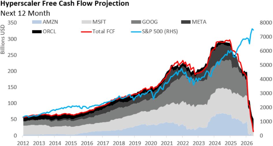
Chart of the Week: Micron’s $41.5B revenue blowout and the OpenAI IPO delay arrived in the same week — two views of the same chart. The AI hardware supply side is confirmed real (HBM booked through 2027, $22B in customer deposits); the demand sustainability question is now live (OpenAI deferring its $1 trillion public offering because the market won’t price a pre-profit AI company at that valuation). This chart explains how both can be true simultaneously: hyperscaler capex has tripled to $725B in 2026 guidance while forward free cash flow approaches zero, the build now self-funding through bond markets and customer deposits rather than operating cash — the week proved both clauses of Friday’s chart caption at once: the market is still pricing optionality, and the infrastructure is already holding obligations.
MIB Weekly Digest Ver. 1.64
For professional investors only. Not investment advice.
© 2026 RecessionALERT.com
MIB Daily: AI Capex Cracks, FOMC Unanimously Hawkish — Enterprise Software Long, Memory Short, Iran Oil Binary at $69 Unresolved
MARKET INTELLIGENCE BRIEF (MIB)
Friday, June 26, 2026
OpenAI may delay its IPO to 2027 — WDC -13%, STX -12%, Nasdaq -1.09% — as markets rotated into enterprise software (MSFT +5.71%, PLTR +5.28%). Kashkari flipped to a 2026 hike, completing a unanimous FOMC hawk chorus; the trade deficit exploded to $105.8B vs. $85B, lifting September cut odds to 55%. LLY +7.13% on EU leukemia approval drove healthcare to a record weekly outperformance. Iran struck a Hormuz vessel but oil fell -2.73%. Trump threatened 100% tariffs on DST nations.
TABLE OF CONTENTS
A. EXECUTIVE SUMMARY
B. MARKET DATA
C. HIGH-IMPACT STORIES (6)
D. MODERATE-IMPACT STORIES (5)
E. ECONOMY WATCH (5)
F. EARNINGS WATCH (0)
G. WHAT’S NEXT
H. CHART OF THE DAY
A. EXECUTIVE SUMMARY -> TOP
Friday exposed a structural fracture in the AI investment thesis: OpenAI’s reported IPO delay to 2027 implicitly signals hardware capex may be front-loaded into a build-out that lacks the revenue model to sustain it — the hardware-to-software rotation that followed (storage/memory −10–13%, enterprise software +5–6%) has lasting valuation implications for data center and semiconductor equities. Simultaneously, Kashkari’s flip to a 2026 hike eliminated the last FOMC dovish voice, shifting the Committee’s operative question from “cut or hold” to “hold or hike” — a structural constraint on long-duration assets. The May trade deficit ($105.8B vs. $85B expected) adds 0.75–1.0 ppts in Q2 GDP drag while paradoxically lifting September cut odds to 55%, creating a bimodal rate path that compresses positioning margins into July. Breadth was constructive: 7 of 11 sectors advanced, with healthcare and defensives leading — this was an AI hardware selloff, not a systemic event.
• OpenAI IPO delay to 2027 reported — WDC −13.17%, STX −12.24%, SNDK −10.46%, TXN −8.46%, NVDA −6% collapsed the Nasdaq −1.09%; enterprise AI software (MSFT +5.71%, PLTR +5.28%, IBM +4.91%) surged as markets repriced AI monetization from hardware capex to recurring software revenue
• Kashkari flips to 2026 hike — joins 9 of 18 FOMC officials projecting at least one hike; Williams delays 2% inflation return to 2028; Goolsbee says inflation is “going the wrong way” — the FOMC is now unanimously hawkish for the first time this cycle
• US trade deficit explodes to $105.8B vs. $85B expected (+27.4% monthly jump) — Q2 GDP net export drag ~0.75–1.0 ppts; September rate cut odds rise to 55% despite concurrent hike signals, creating a bimodal rate path
• LLY +7.13% after EU CHMP recommends Jaypirca for all-line CLL; FDA decision expected H2 2026; healthcare (+2.68%) posts record weekly outperformance vs. S&P 500 (+7.59% WoW)
• Iran drone strikes Hormuz vessel, Trump declares ceasefire violation — WTI still −2.73% to $69.96; markets weigh deal durability over incident; binary escalation risk elevated over 48–72 hours
• Trump threatens 100% tariffs on all countries with digital services taxes (France, UK, India, Spain, Austria) — GOOG −2.19%; reintroduces acute trade war risk against allied partners at a moment of normalization
1. AI Monetization Bifurcation — The market has cleanly split AI investing into two categories with opposite risk profiles: hardware capex (memory, storage, GPUs) is de-risking on demand uncertainty as the OpenAI IPO delay questions the revenue sustainability of the AI infrastructure build-out; enterprise software (MSFT, PLTR, IBM) is re-rating on revenue certainty as AI monetization is demonstrated through recurring cloud and contract revenue. This divergence — hardware −10–13% vs. software +5–6% in a single session — has structural portfolio allocation implications that extend beyond a one-day rotation trade.
2. Bimodal Rate Path Compresses Q3 Positioning Margins — The FOMC has reached unanimous hawkish consensus (Kashkari, Williams, Goolsbee, Warsh all signaling hold-or-hike) while the same day’s data (trade deficit blowout, Michigan near record low, September cut odds at 55%) argues for easing. This bimodal rate regime — where a single week’s data simultaneously supports a hike and a cut — maximizes volatility around every July data print (CPI July 15, PCE July 31). Portfolio positioning must account for both tails; the “soft landing” middle scenario carries the narrowest probability band.
3. Iran Deal Binary Unresolved at $69 Oil — Oil’s continued decline through a vessel strike and “ceasefire violation” declaration confirms markets are pricing deal durability as the base case. But the binary is live: any US escalatory response re-restricts 1.0–1.5M bpd of Iranian crude and produces a rapid $5–10 recovery from current $69 WTI — the energy sector carries asymmetric upside risk that no fundamental model fully captures at this juncture.
B. MARKET DATA -> TOP
Healthcare (+2.68%) surged on EU approval of Eli Lilly’s leukemia therapy, while Technology (-0.96%) was dragged lower by a 10–13% collapse in storage and memory names — an ongoing Korean market contagion and OpenAI’s reported IPO delay threatening AI data-center capex timelines. The S&P 500 closed essentially flat (-0.06%) and NYSE actually gained +0.33%, as defensive rotations offset the Nasdaq 100’s -1.09% drop — this was a sector-specific selloff, not a systemic one. Oil slid -2.73% on continued Iran-deal supply expectations despite a vessel being struck off Oman, while gold gained +0.99% as a precautionary safe-haven. With Technology down -5.54% on the week but its 3-month lead (+27.97%) still substantial, the rotation into healthcare and defensives bears watching into Q3.
CLOSING PRICES – Friday, June 26, 2026:
MAJOR INDICES
Small-cap outperformance versus mega-cap tech is now an entrenched 7-session trend: Russell 2000 has returned +2.85% over the past 10 sessions versus the S&P 500’s -0.55%, a 3.4-percentage-point spread driven by domestic cyclical resilience while AI-exposed mega-caps bear the correction. Today reinforced that divergence — the Nasdaq (-1.09%) bore the brunt of the storage/AI selloff while the Russell (-0.18%) and NYSE (+0.33%) held firm. No Dow Theory signal fires: DJIA sits within 0.3% of its 10-session high while DJTA is 3.4% below — not yet the 5% non-confirmation threshold, but the transport gap is widening.
| Index | Close | Change | %Move | Why It Moved |
|---|---|---|---|---|
| S&P 500 | 7,353.15 | -4.34 | -0.06% | Defensive/healthcare gains offset Nasdaq-led tech decline; effectively flat close |
| Dow Jones | 51,865.52 | -55.10 | -0.11% | Blue-chip composition partially buffered tech selloff; industrials (-1.38%) the main drag |
| DJ Transportation | 21,822.4 | -110.1 | -0.50% | Freight/logistics names softened on oil decline and macro growth uncertainty |
| Nasdaq 100 | 29,118.24 | -322.08 | -1.09% | Storage/memory names collapsed 10–13% on Korean market contagion and OpenAI IPO delay; software AI names partially offset |
| Russell 2000 | 3,002.57 | -5.29 | -0.18% | Small-caps resilient vs mega-cap tech; domestic exposure less AI hardware-dependent; 7-session outperformance streak continues |
| NYSE Composite | 23,689.23 | +78.51 | +0.33% | Broad market positive; healthcare/defensive/REIT rotation outweighed tech drag; breadth constructive |
VOLATILITY & TREASURIES
VIX falling -2.70% while equities barely moved confirms a narrow, sector-specific selloff — genuine fear would show up in VIX even on mild down-days. Yields fell modestly (10Y -1.6 bps, 2Y -2.7 bps) with the short end leading, a mild rate-cut-friendly signal; the 2Y–10Y spread ticked to +27.9 bps from +26.0 bps yesterday, a slight steepening. DXY -0.11% moved with yields — no safe-haven dollar bid, confirming bond markets are declining to validate the tech selloff as a systemic risk event.
| Instrument | Level | Change | Why It Moved |
|---|---|---|---|
| VIX | 18.38 | -0.51 (-2.70%) | Narrow tech-specific selloff; options market not pricing systemic risk despite Nasdaq -1.09% |
| 10-Year Treasury Yield | 4.373% | -1.6 bps | Modest safe-haven demand; Iran Strait vessel incident; rate-cut expectations persisting |
| 2-Year Treasury Yield | 4.094% | -2.7 bps | Short end fell more than long end; mild dovish Fed signal; yield curve steepened slightly |
| US Dollar Index (DXY) | 101.32 | -0.11 (-0.11%) | Mild dollar weakness tracking yield decline; no flight-to-safety dollar bid |
COMMODITIES
Gold (+0.99%) and precious metals advanced as the Oman vessel incident maintained a thin safe-haven bid despite oil’s decline. Copper (+0.92%) diverged positively from WTI (-2.73%), confirming the energy weakness is supply-driven rather than a global demand collapse — industrial metals do not see demand destruction in an Iran sanctions-relief scenario. Bitcoin (+0.35%) remained a mild risk proxy, tracking broadly with equities rather than generating its own narrative.
| Asset | Price | Change | %Move | Why It Moved |
|---|---|---|---|---|
| Gold | $4,087.85/oz | +$40.25 | +0.99% | Safe-haven bid; vessel struck off Oman; oil decline and Strait of Hormuz uncertainty |
| Silver | $58.505/oz | +$0.144 | +0.25% | Co-movement with gold; modest precious metals advance |
| Copper | $6.1300/lb | +$0.0560 | +0.92% | AI/electrification demand narrative intact; industrial metals diverge from oil weakness |
| Platinum | $1,619.00/oz | +$16.00 | +1.00% | Precious metals broadly supported; safe-haven and industrial demand crossover |
| Bitcoin | $59,667.0 | +$208.0 | +0.35% | Mild risk-proxy tracking; no crypto-specific catalyst; decoupled from tech hardware selloff |
ENERGY
WTI and Brent fell in near-lockstep (-2.73%/-2.89%) — a tight spread confirms globally supply-driven pressure from Iran Strait of Hormuz normalization rather than a regional disruption; rising shipping through the Strait is the primary driver. A vessel struck by a projectile off Oman added uncertainty but failed to reverse the trajectory. Dutch TTF gained +1.11% in dollar terms while Henry Hub fell -0.24% — European gas continues to trade at a significant premium, reflecting the Iran deal’s limited effect on European supply chains.
| Asset | Price | Change | %Move | Why It Moved |
|---|---|---|---|---|
| Crude Oil (WTI) | $69.96/bbl | -$1.96 | -2.73% | Iran Strait of Hormuz supply normalization; rising shipping activity through strait despite Oman incident |
| Crude Oil (Brent) | $73.32/bbl | -$2.18 | -2.89% | Same supply normalization factors; near-lockstep with WTI confirms global rather than regional driver |
| Natural Gas (Henry Hub) | $3.287/MMBtu | -$0.008 | -0.24% | Near-neutral; summer demand normal; unaffected by Iran deal dynamics |
| Natural Gas (Dutch TTF) | $13.61/MMBtu | +$0.15 | +1.11% | European gas premium persists; Iran deal has limited effect on European supply chains; EUR/USD +0.15% added to dollar-denominated price |
S&P 500 SECTORS
Healthcare is the clear rotation beneficiary: +2.68% today, +7.59% this week, +7.74% this month — the only sector with sustained strength across all near-term horizons. Technology (+27.97% 3M) is the mirror image: a multi-quarter dominance story cracking badly, -5.54% this week and -0.96% today. Energy (-12.19% 3M) declined again (-0.47%) despite being the YTD leader (+19.46%) — the Iran-deal supply shock is structurally repricing the sector lower into its second consecutive month of losses.
| Sector | 1-Day | 1-Week | 1-Month | 3-Month | 6-Month | YTD | 12-Month |
|---|---|---|---|---|---|---|---|
| Healthcare | +2.68% | +7.59% | +7.74% | +10.79% | +3.91% | +4.68% | +21.25% |
| Consumer Cyclical | +1.59% | -2.42% | -7.13% | +4.32% | -8.48% | -6.41% | +3.99% |
| Real Estate | +1.54% | +4.02% | +2.35% | +12.33% | +11.63% | +11.62% | +10.97% |
| Consumer Defensive | +0.97% | +1.90% | -0.08% | +3.28% | +8.30% | +8.29% | +6.71% |
| Utilities | +0.78% | +3.53% | +1.42% | +1.77% | +7.97% | +8.18% | +17.01% |
| Financial | +0.29% | +0.07% | +4.08% | +11.98% | +0.38% | +1.60% | +12.86% |
| Communication Services | -0.10% | -5.43% | -11.09% | +7.11% | -3.98% | -3.66% | +17.98% |
| Basic Materials | -0.23% | -4.22% | -5.62% | +3.09% | +7.09% | +9.64% | +37.27% |
| Energy | -0.47% | -0.45% | -6.26% | -12.19% | +19.99% | +19.46% | +26.95% |
| Technology | -0.96% | -5.54% | -2.87% | +27.97% | +16.70% | +17.91% | +34.77% |
| Industrials | -1.38% | -2.71% | +1.65% | +12.16% | +15.67% | +17.68% | +28.41% |
TOP MEGA-CAP MOVERS:
GAINERS
| Company | Ticker | Close | Change | Why It Moved |
|---|---|---|---|---|
| Lilly (Eli) & Co | LLY | $1,208.12 | +7.13% | EU backed use of its leukemia therapy (BTK inhibitor); healthcare sector leadership; pulled defensive pharma names higher |
| Microsoft Corp | MSFT | $372.97 | +5.71% | Enterprise AI software rotation; Azure cloud growth narrative; software AI names benefited as storage/hardware AI complex sold off |
| Palantir Technologies Inc | PLTR | $112.93 | +5.28% | AI software/data analytics rotation; enterprise and government AI demand; hardware-to-software AI shift on OpenAI IPO delay |
| International Business Machines Corp | IBM | $271.63 | +5.17% | Enterprise AI software rotation; cloud and AI services; benefited from pivot away from hardware AI capex plays |
| Abbvie Inc | ABBV | $253.35 | +4.20% | Healthcare sector rotation; LLY EU approval lifted broader pharma/biotech segment; defensive positioning |
DECLINERS
| Company | Ticker | Close | Change | Why It Moved |
|---|---|---|---|---|
| Western Digital Corp | WDC | $586.45 | -13.17% | Multi-day correction from record highs; Korean memory market contagion (KOSPI -10%); AI data center storage demand uncertainty on OpenAI IPO delay |
| Seagate Technology Holdings Plc | STX | $899.90 | -12.24% | Storage sector contagion; HDD demand uncertainty; Korean DRAM/NAND market correction spillover |
| Sandisk Corp | SNDK | $2,090.71 | -10.46% | NAND flash memory correction; WDC NAND spinoff facing same Korean supply-chain contagion; AI capex uncertainty |
| Texas Instruments Inc | TXN | $285.42 | -8.46% | Semiconductor sector selloff; analog/embedded chip demand concerns amid AI capex uncertainty and Korean market contagion |
| Micron Technology Inc | MU | $1,132.33 | -6.69% | Post-Q3 FY2026 blowout earnings “sell the news” correction (reported Jun 24: record $41.5B revenue, 85% margins); Korean DRAM contagion continues |
C. HIGH-IMPACT STORIES -> TOP
BEARISH
1. OpenAI Delays IPO to 2027 as AI Capex Uncertainty Triggers Semiconductor Selloff — Nasdaq -1.09%, WDC -13%, STX -12%, SNDK -10%, NVDA -6%
The core facts:Reports from The New York Times and Bloomberg, citing OpenAI advisers, indicate the company is weighing a delay of its planned public offering until 2027, citing recent tech stock volatility and insufficient market appetite to support CEO Sam Altman’s stated $1 trillion valuation target. OpenAI’s hesitation was reportedly triggered in part by SpaceX’s post-IPO decline of more than 20% from its June 12 peak, which undermined confidence in investor appetite for high-growth, pre-profit AI assets at extreme valuations. The report triggered a broad semiconductor selloff: WDC -13.17%, STX -12.24%, SNDK -10.46%, TXN -8.46%, MU -6.69%, NVDA -6%; AMD also fell sharply. SoftBank — which holds approximately 13% of OpenAI via a cumulative ~$65 billion investment — fell more than 12%. The Nasdaq Composite closed -1.09%, its second consecutive session of losses; the S&P 500 was approximately -0.06%, confirming the selloff was concentrated in AI-exposed tech rather than the broad market.
Why it matters:The OpenAI IPO delay reframes the “AI capex supercycle” narrative that has driven semiconductor valuations to record levels. The specific concern is structural: OpenAI’s hardware consumption is the downstream demand anchor for HBM, NAND, server storage, and GPU supply chains. If OpenAI is pulling back its IPO timeline because of valuation uncertainty, it implicitly signals that AI infrastructure spending may be front-loaded into a speculative build-out that lacks the proven revenue model to sustain it at current scale. For investors, WDC -13% and STX -12% on a single unconfirmed report suggest the storage and memory complex was priced for perfection and is acutely sensitive to demand signal deterioration. SoftBank’s -12% is a direct mark-to-market consequence of its $65B OpenAI position. The divergence between hardware AI names (down 7–13%) and enterprise AI software names (MSFT +5.71%, PLTR +5.28%, IBM +4.91%) is the market’s immediate re-pricing of where AI monetization actually resides — in software revenue streams, not capital expenditure cycles.
What to watch:Any direct OpenAI statement confirming or denying the 2027 timeline; Micron’s Q4 FY2026 results (~September 2026) as the first hard data test of whether the IPO delay translates to actual demand reduction from the $50B guidance; NVIDIA’s next earnings call for explicit hyperscaler capex commentary post-IPO delay report.
BULLISH
2. Eli Lilly’s Jaypirca Gets EU CHMP Recommendation for All-Line CLL — LLY +6%, Healthcare Posts Record Weekly Outperformance vs. S&P 500
The core facts:The European Medicines Agency’s Committee for Medicinal Products for Human Use (CHMP) issued a positive opinion recommending approval of Lilly’s Jaypirca (pirtobrutinib) for adults with chronic lymphocytic leukemia (CLL) across all lines of therapy — including patients who have previously received BTK inhibitor treatment. The recommendation is backed by Phase 3 data from the BRUIN CLL-313 and BRUIN CLL-314 trials. The European Commission is expected to issue a final decision within 1–2 months. Lilly has separately submitted the CLL data to the FDA, with a US regulatory decision expected in the second half of 2026. LLY rose approximately 6% to approximately $1,208 on Friday. ABBV gained approximately 4.20% on sector rotation tailwinds. The healthcare sector (XLV) posted its strongest weekly performance relative to the S&P 500 on record — gaining approximately +2.68% on the day, +7.59% for the week, and +7.74% for the month.
Why it matters:The Jaypirca CHMP recommendation extends Lilly’s oncology franchise into commercially important territory: “all lines” CLL approval removes the prior constraint limiting Jaypirca to later-line use after BTK inhibitor failure, and first-line CLL eligibility substantially expands the addressable market. The EU recommendation validates the Phase 3 data supporting the FDA’s parallel US filing, creating a regulatory risk-reduction catalyst as investors price the probability of a US approval in H2 2026. The broader healthcare dynamic is equally significant: healthcare’s record weekly relative outperformance vs. S&P 500 reflects a structural rotation driven by GLP-1 momentum, oncology pipeline catalysts, and defensive positioning amid AI hardware volatility. Healthcare simultaneously offers defensive characteristics (lower rate sensitivity vs. growth tech) and growth optionality (GLP-1, oncology) — a rare configuration in the current rate environment.
What to watch:FDA decision on Jaypirca CLL filing in H2 2026 as the US market entry catalyst; Lilly’s Q2 2026 earnings (late July) for Mounjaro/Zepbound revenue guidance and Jaypirca launch trajectory; European Commission final approval (within ~2 months) as the formal EU commercial trigger.
UNCERTAIN
3. Iran Drone Strikes Cargo Vessel in Hormuz — Trump Alleges Ceasefire Violation; IMO Pauses Evacuation Plan; WTI -3.74%, Brent -4.34%
The core facts:Iran’s military conducted a drone strike on a Singapore-flagged cargo vessel in the Strait of Hormuz area near the coast of Oman on June 26, according to a US official. The UK Maritime Trade Operations confirmed the vessel reported no casualties and no environmental damage. Following the attack, the International Maritime Organization temporarily paused its ongoing vessel evacuation plan to reassess safety conditions. President Trump publicly stated that “Iran had violated the ceasefire with drone attacks,” characterizing it as “a foolish violation of our Ceasefire Agreement.” Despite the military escalation, WTI crude oil settled down 3.74% to approximately $69.23/bbl and Brent settled down 4.34% to approximately $71.99/bbl, as overall tanker traffic through the Strait of Hormuz continued to increase following the US–Iran accommodation reached over the past week — oil has fallen approximately 22% over the past month and is down four consecutive weeks.
Why it matters:The vessel strike introduces meaningful ambiguity about whether the US–Iran accommodation is durable or represents a temporary commercial window that Iran can selectively open and close. Trump’s explicit “ceasefire violation” language — in public, specific terms — creates two binary scenarios for energy markets: (1) the US responds with escalatory military or sanctions action, Iranian crude access (potentially 1–1.5 million bpd) is re-restricted, and WTI recovers sharply from $69, which fully prices a functional deal; (2) the strike is assessed as an isolated provocation outside official Iranian policy, the accommodation holds, and WTI continues at $68–72 or lower. Markets are currently weighting scenario (2) — oil fell further despite the attack — but the IMO evacuation pause and Trump’s “ceasefire violation” declaration introduce acute headline risk. Any escalatory US response would produce a rapid $5–10 oil price reversal from current levels. For energy equities: XLE has declined four consecutive weeks pricing the deal; a deal fracture now has an explicit triggering event. For safe-haven assets: the strike provided brief support for gold (+1.13%) and limited the dollar’s decline.
What to watch:US government official response over the next 48–72 hours — whether military or sanctions action follows Trump’s “ceasefire violation” declaration; daily tanker tracking data through Hormuz as the continuous supply flow indicator; the 60-day sanctions waiver expiration timeline as the hard binary event for Iranian crude market access.
UNCERTAIN
4. US Advance Goods Trade Deficit Blows Out to $105.8B vs. $85B Expected — Net Export Drag Sharpens Q2 GDP Risk; September Rate Cut Odds Jump to 55%
The core facts:The US Census Bureau released the Advance Goods Trade Balance for May 2026 on June 26: -$105.8 billion versus -$85.0 billion consensus and -$83.0 billion prior — a $20.8 billion monthly miss (+27.4% deficit jump). Exports declined -5.4% and imports increased +3.6%. Tariff front-running — businesses pulling forward imports ahead of potential tariff increases — is the dominant explanation for the import surge. Net exports are now on track to subtract approximately -0.75 to -1.0 percentage points from Q2 2026 GDP. The market reaction: September rate cut probability moved from approximately 45% to approximately 55% on the data — the first time September has become a base-case (>50%) cut scenario in recent months, even as Kashkari simultaneously projected a 2026 rate hike (see Story 5), creating a bimodal rate path in bond markets.
Why it matters:The $105.8B deficit is a textbook tariff distortion: when businesses front-run tariffs by pulling forward imports, the trade balance deteriorates mechanically, dragging GDP even as underlying domestic demand may be unaffected. The result is a GDP miss caused by policy that was intended to improve the trade balance — precisely the perverse dynamic that economists flagged when Q1’s headline GDP beat (2.1%) was driven entirely by import compression from the prior quarter’s tariff front-running. The September rate cut repricing to 55% is structurally significant because it directly contradicts Kashkari’s concurrent hike projection — bond markets are simultaneously pricing a trade-deficit-driven cut scenario AND a hike risk scenario. This bimodal positioning explains the anomalous short-end Treasury behavior (2-year yields falling despite a hike signal) and compresses the margin for policy error. For equity portfolio managers: the divergence between a widening trade deficit, a hawkish Fed, and markets near all-time highs concentrates volatility risk in the July data calendar — PCE, CPI, retail sales, and trade data all arrive within six weeks.
What to watch:Atlanta Fed GDPNow Q2 update within 48 hours of this release for quantification of the net export drag; July 15 CPI and July 31 PCE as the convergence data points determining whether September is a live cut or hike; June trade balance (balance of goods and services) to confirm whether May’s $105.8B is a one-month tariff anomaly or trend.
BEARISH
5. Kashkari Flips from Cut to Hike — Historically Dovish Fed Voice Joins 9 FOMC Officials Projecting ≥1 Rate Hike in 2026; FOMC Now Unanimously Hawkish
The core facts:Minneapolis Federal Reserve President Neel Kashkari said at the Aspen Ideas Festival on June 26 that he now expects one rate increase in 2026, reversing his March projection of one rate cut. Kashkari is historically among the FOMC’s most dovish regional presidents — his reversal carries significant signaling weight. The June 17 FOMC dot plot had already shown 9 of 18 officials projecting at least one 2026 rate hike, with the median forecast rising to 3.8% from 3.4% in March. Kashkari specifically cited AI and data center capital expenditure as a near-term inflation driver alongside tariffs. Fed Governor Williams (June 25) extended the 2% inflation return timeline to 2028; Goolsbee characterized inflation as “going the wrong way.” Together, June 25–26 Fed communication represents a full Committee sweep toward tightening bias — no dovish dissent voice remains. Polymarket 2026 hike probability sits at approximately 52%.
Why it matters:Kashkari’s flip eliminates the last visible “dovish dissent” within the FOMC. When the Committee’s historically most dovish public voice endorses a hike, the distribution of plausible outcomes has shifted materially — the question is no longer “cut or hold” but “hold or hike.” This has structural implications for all long-duration assets (equities, REITs, utilities, long-dated bonds) that have been rebounding from early 2026 underperformance in anticipation of eventual rate relief. Kashkari’s explicit identification of “AI and data center capex” as an inflation driver adds an unusual dimension: tech sector investment — the primary driver of equity market performance in 2024–2026 — is now explicitly identified by a Fed official as a near-term inflationary force. This creates a self-referential pressure: AI capex drives inflation, inflation justifies hikes, hikes compress the multiples that justified AI capex investment, which reduces AI capex, which eventually reduces the inflation driver. The complete Fed communication arc — Chair Warsh drops easing bias (June 17), Williams “unquestionably elevated” (June 25), Goolsbee “going the wrong way” (June 25), Kashkari flips to hike (June 26) — represents an extraordinary consensus shift in under two weeks.
What to watch:Fed Chair Warsh’s next public statement for explicit September language; September FOMC (September 15–16) as the first live hike window; CME FedWatch probability above 50% for September hike as the equity multiple re-pricing threshold.
BEARISH
6. Trump Threatens Immediate 100% Tariffs on All Goods from Countries Imposing Digital Services Taxes — Meta, Alphabet, Amazon Directly Exposed
The core facts:President Trump announced on June 26 that the US would immediately impose 100% tariffs on all goods imported from any country that levies a “digital services tax” on US technology companies. Trump’s statement: “any Country that imposes such a Tax will immediately be met with a 100% TARIFF on any and all Goods sent to the United States of America.” Digital services taxes — designed to tax large US tech platforms on local revenues where they lack a physical taxable presence — are currently in effect in more than a dozen countries including France, Italy, Spain, the United Kingdom, India, and Austria. The primary exposed companies are Meta (Facebook/Instagram/WhatsApp), Alphabet (Google/YouTube/Search), and Amazon (AWS/marketplace), all of which operate at scale in digital services tax jurisdictions. GOOG fell -2.19% on the day. The legal basis for an “immediate” 100% tariff through executive action without a USTR investigation was not specified in Trump’s announcement.
Why it matters:A 100% tariff on all goods from France, the UK, India, Spain, and other digital services tax jurisdictions would represent the broadest single-day US trade escalation since the April 2025 universal tariff announcement — this time explicitly targeting allied trading partners in retaliation for taxation of US tech companies. The digital services tax issue has been a persistent US–Europe friction point since 2019; Trump’s 100% tariff language (versus the 25% retaliatory framing of prior administrations) represents qualitative escalation in both magnitude and speed. For US tech companies: digital services taxes are primarily a cost-center (typically 2–5% levies on local revenues) but the precedent that the US will impose country-wide 100% goods tariffs in retaliation creates an existential risk for any country considering DST expansion — this is explicitly coercive trade policy. For broader markets: the threat reintroduces acute tariff uncertainty at a moment when risk assets were beginning to price in trade normalization following the US–Iran oil deal and partial US–China tariff rollback discussions. European luxury goods (LVMH, Hermès), UK defense exporters, and Indian IT services companies are among the sectors most exposed to a 100% retaliatory regime.
What to watch:European Union and France’s formal response — whether they expand, pause, or rescind DST plans in response to Trump’s threat; USTR’s identification of the statutory authority cited for immediate 100% tariff imposition; Alphabet and Meta Q2 2026 earnings (mid-July) for commentary on international revenue risk from DST expansion.
D. MODERATE-IMPACT STORIES -> TOP
BULLISH
7. SpaceX and CoreWeave Join Russell 1000 in Annual Reconstitution — $22–27B in Forced Mechanical Index Buying Triggered at Friday Close
The core facts:FTSE Russell’s annual index reconstitution took effect at the close of trading on June 26, adding SpaceX (SPCX) and CoreWeave (CRWV) to the Russell 1000 and Russell 3000 under the exchange’s newly adopted fast-track entry rule, which allows companies with investable market caps above the Russell Top 500 breakpoint to enter Russell indexes after just five trading days of listing. SpaceX, which debuted on Nasdaq on June 12 (+19.34% first-day), enters with a multi-hundred-billion dollar market capitalization. Combined mechanical buying from Russell inclusion and parallel MSCI fast-track inclusion is estimated at $22–27 billion in forced institutional purchases of SPCX at Friday’s closing prices. SPCX gained approximately +1.5% during the session on anticipation of the closing buy imbalance. CoreWeave (CRWV), the GPU cloud computing company that went public in March 2026, joins simultaneously. Note: S&P 500 inclusion requires GAAP profitability, which SpaceX lacks — S&P 500 entry is not part of this event.
Why it matters:SpaceX’s Russell 1000 inclusion is one of the largest-ever single-name forced index buying events. Every ETF and passive fund tracking Russell 1000, Russell 3000, and MSCI US indexes must acquire SPCX proportional to its index weight — creating a mechanical demand event independent of fundamental analysis or price discovery. The $22–27 billion in forced buying is a one-session price catalyst that may produce a gap between SPCX’s post-inclusion price and fundamental valuation, consistent with the well-documented “index inclusion premium.” CoreWeave’s simultaneous entry provides a second AI infrastructure name in these benchmarks, permanently institutionalizing AI infrastructure as a passive allocation. The combination creates an ongoing structural demand for both names beyond the one-session buying event: all future passive fund flows will include SPCX and CRWV allocations proportional to their index weights.
What to watch:SPCX’s first post-inclusion session (Monday June 29) for the reversal or follow-through pattern characteristic of index inclusion events; MSCI official fast-track inclusion confirmation as the second tranche of forced buying; Nasdaq 100 inclusion timeline requiring a later review given market cap composition rules.
BULLISH
8. Enterprise AI Software Rallies as Hardware Capex Risk Rises — IBM JP Morgan Upgrade, MSFT +5.71%, PLTR +5.28%, IBM +4.91%
The core facts:Enterprise AI software stocks outperformed sharply on June 26 as the OpenAI IPO delay report triggered rotation away from hardware-linked AI names. Microsoft (MSFT) gained 5.71%, recovering significant ground from Thursday’s -3.46% decline. Palantir Technologies (PLTR) gained 5.28%. IBM gained 4.91% after J.P. Morgan upgraded the stock from Neutral to Overweight, raising its price target, with analysts citing IBM’s hybrid-cloud OpenShift platform, AI-driven container adoption, and the fact that software generates approximately two-thirds of IBM’s consolidated profits despite being a minority of total revenue. Microsoft’s AI business has reached a $37 billion annualized run rate (+123% year-over-year); Azure grew 31% in the most recent quarter. The three names combined represent meaningful S&P 500 and Dow Jones index weight.
Why it matters:The enterprise software outperformance on June 26 encodes a direct market thesis: if AI infrastructure capex timelines are extending and uncertain (OpenAI delay), then the winners are companies monetizing AI through recurring software revenue rather than hardware-dependent capex cycles. Microsoft’s Azure, IBM’s hybrid-cloud platform, and Palantir’s AI deployment contracts are revenue-generating today rather than contingent on future capex build-out. The JP Morgan IBM upgrade adds fundamental validation: an analyst is explicitly recommending IBM because its software mix and hybrid-cloud positioning are undervalued relative to its peers. MSFT’s 5.71% single-day recovery (full round-trip from Thursday’s -3.46% hardware-cost-driven selloff) signals that the market’s framing is shifting from “AI hardware costs” to “AI enterprise monetization.” For portfolio managers, the rotation creates a clear tactical pair trade: long enterprise AI software (MSFT, IBM, PLTR, NOW, ADSK) versus reduced exposure to AI hardware capex names (storage, memory, data center construction).
What to watch:Microsoft Azure constant-currency growth guidance at next earnings (late July) as the revenue inflection test for the software-over-hardware thesis; IBM’s hybrid-cloud bookings in Q2 2026 results; PLTR’s next government and commercial contract pipeline update.
UNCERTAIN
9. Michigan Consumer Sentiment Final June 49.5 — 5-Year Inflation Expectations Ease to 3.3% from Record 3.9%; Consumer Confidence Stabilizes After Record Low
The core facts:The University of Michigan’s final Consumer Sentiment for June 2026 came in at 49.5 — slightly below the 50.0 consensus but materially above the May 2026 record low of 44.8. The 5-year inflation expectations reading eased to 3.3% from the prior 3.9%, while near-term 1-year expectations fell slightly to 4.6% from 4.8% prior. The 5-year reading is the Federal Reserve’s most closely watched consumer inflation gauge and a primary input into the “inflation de-anchoring” risk assessment. The June headline reading represents a 4.7-point recovery from the record low — the largest single-month rebound in the survey’s recent history.
Why it matters:The Michigan 5-year reading easing from 3.9% to 3.3% is a marginally cut-supportive signal that directly conflicts with Kashkari’s concurrent hike narrative: if consumers believe inflation will moderate over five years, the risk of a self-sustaining wage-price spiral declines, giving the Fed more flexibility to respond to growth weakness without triggering a credibility crisis. This creates an unusual analytical fork: Kashkari projects a hike based on backward-looking realized inflation (Core PCE 3.4%, wages +0.7%), while the 5-year expectations easing suggests forward-looking consumer inflation psychology is actually improving. The headline 49.5 recovery from 44.8 adds to this picture — May’s record low was set at peak tariff-driven pessimism; any stabilization signals that consumer confidence has not collapsed further, which is important for Q3 spending trajectory. The confluence of easing 5-year expectations (dovish signal), rising September cut odds (dovish), and Kashkari’s hike flip (hawkish) represents precisely the data-dependent bimodal rate regime that maximizes near-term equity volatility — markets cannot price a single scenario.
What to watch:July Michigan preliminary reading (late July) for directional confirmation of the 3.9%→3.3% easing in 5-year expectations; Core CPI July 15 and Core PCE July 31 as the hard data tests determining whether the rate market resolves the cut vs. hike binary.
UNCERTAIN
10. Baker Hughes US Rig Count +10 — Largest Weekly Gain in Four Years — Supply Expansion Continues at $69 WTI
The core facts:Baker Hughes released its weekly US rig count on June 26, showing a net increase of 10 active rigs — the largest single-week gain in approximately four years — bringing total US active rigs to approximately 500. The increase occurred despite WTI crude oil trading near $69/bbl, approximately a 22-month low and 22% below its level one month ago. The energy sector (XLE) was down approximately 0.47% on the day and -12.19% over the past three months. The rig count increase spanned both oil and natural gas categories.
Why it matters:Rising US rig counts at $69/bbl runs counter to the typical price-volume response and requires explanation. US shale operators are likely sustaining activity because: (1) rigs were booked and wells hedged at $75–80+ prices before the Iran deal repriced the market; (2) multi-year development programs cannot be economically suspended at a single quarter’s spot price; (3) forward hedging programs on many wells maintain sufficient unit economics at current prices. For oil markets, the supply implication compounds the downward oil price pressure: more US rigs at $69 means incremental US production volume is increasing precisely when Iranian crude is also returning to global markets. The dual supply headwind — Hormuz normalization plus US rig count expansion — makes a sustained WTI recovery above $75 structurally harder without a major supply disruption. For energy services companies (SLB, HAL, BKR), the rig count increase is a positive demand signal even in a declining price environment. The divergence — XLE equity prices down 12% while operational activity expands — reflects the market discounting near-term margin compression from low realized prices even as operators maintain production growth.
What to watch:Next week’s rig count for continuation confirmation; WTI holding below $70 as the sustainability test for current drilling programs; SLB and HAL Q2 2026 earnings (mid-July) for North American activity level guidance.
BEARISH
11. Bitcoin Spot ETFs Record ~$1.35B in Weekly Outflows — Institutional Redemptions Deepen as Real Rate Hike Risk Undermines Non-Yield Crypto Thesis
The core facts:US-listed Bitcoin spot ETFs recorded approximately $1.35 billion in net outflows for the week ending June 26 — among the largest weekly redemption totals since the category launched in January 2024. Bitcoin traded essentially flat on Friday (-0.05%) after a prolonged multi-session decline that has left the cryptocurrency significantly below its 2026 highs. The macro drivers cited by analysts: Core PCE at 3.4% (June 25), Kashkari’s June 26 hike projection, and rising real yields that increase the opportunity cost of holding non-yielding crypto assets relative to Treasury bills and money market funds now yielding 4%+. Bitcoin ETF holders who entered at higher prices are increasingly carrying mark-to-market losses, generating incremental redemption pressure.
Why it matters:The $1.35 billion in weekly ETF outflows is a qualitative shift from the net-positive inflow dynamic that characterized Bitcoin ETF behavior through the first five months of 2026. Spot Bitcoin ETFs became the dominant institutional access vehicle for the asset after their January 2024 launch — cumulative inflows through April 2026 reportedly exceeded $50 billion. Meaningful weekly redemptions signal that institutional allocators are actively exiting, not just pausing. The rate environment is the key macro driver: Bitcoin’s “digital gold” narrative — the central bull case for 2024–2025 — depends on low real yields diminishing the relative attractiveness of yield-bearing alternatives. With the Fed signaling potential 2026 hikes and Core PCE above 3%, real yields are rising, directly undermining the non-yield Bitcoin allocation rationale. The $1.35B outflow figure also has a secondary equity market read-through: institutional funds carrying Bitcoin ETF losses face potential portfolio rebalancing pressure, creating indirect contagion to other risk assets in portfolios where Bitcoin was a high-conviction position. The Iran geopolitical escalation (vessel attack, Trump ceasefire violation claim) notably failed to provide Bitcoin with a safe-haven bid — gold gained +1.13% on the same news, confirming Bitcoin’s decoupling from traditional store-of-value dynamics in rising rate environments.
What to watch:Next week’s Bitcoin ETF flow data for whether outflows accelerate; September FOMC rate path as the primary macro determinant of crypto allocation sentiment; any major institutional or corporate treasury announcement of Bitcoin reduction as a position-size signal.
E. ECONOMY WATCH -> TOP
The week’s macro picture splits between tariff-distorted trade flows and a Fed signaling no retreat on rates. Today’s advance goods trade deficit blew out to -$105.8B (vs -$85B expected) — a potential -0.75% Q2 GDP drag that moved September cut odds from 45% to 55%. That dovish tilt runs directly into FOMC messaging: Kashkari flipped his dot to a hike, Williams extended his 2% inflation timeline to 2028, and both cited broad, durable price pressures. Against that backdrop, the week’s most constructive reads — consumer sentiment bouncing from May’s record low (44.8 → 49.5) and 5-year inflation expectations easing to 3.3% — look credible but fragile. The central tension: markets pricing a September cut while the Fed signals hold-or-hike.
Goods Trade Deficit Explodes to $105.8B in May — Biggest Miss in Years, Q2 GDP Under Threat (Census Bureau, June 26, 2026)
What they’re saying:The advance goods trade deficit widened sharply to $105.8 billion in May — a 27.4% jump from April’s $83.0 billion and well beyond the $85 billion consensus. Exports fell 5.4% ($11.8 billion), led by declines in industrial supplies, while imports rose 3.6% ($10.9 billion). The miss versus expectations was $20.8 billion, one of the largest single-month surprises on record.
The context:The blowout deficit reflects tariff front-running distortions extending into May, as importers rush goods ahead of expected escalation. Net exports are now on track to shave roughly 0.75 percentage points from Q2 real GDP — pressuring Atlanta Fed’s GDPNow (2.5% as of June 25) ahead of the July 1 update. Markets repriced immediately: federal funds futures moved September rate cut odds from 45% to 55%, as the trade shock refocuses attention on slowing growth rather than sticky inflation.
What to watch:Atlanta Fed GDPNow update Wednesday July 1 (will incorporate today’s trade data); advance retail inventories June 30; Q2 GDP advance release (late July).
Michigan Consumer Sentiment Bounces From Record Low But Misses at 49.5; 5-Year Inflation Expectations Ease to 3.3% (University of Michigan, June 26, 2026)
What they’re saying:The University of Michigan Consumer Sentiment Index final reading for June came in at 49.5 — up 10.5% from May’s record low of 44.8, but just short of the 50.0 consensus. The split was notable: Current Conditions missed (47.7 vs 48.9 expected) while Consumer Expectations slightly beat (50.7 vs 50.5). Long-run 5–10 year inflation expectations fell to 3.3% (vs 3.4% expected; prior 3.9%), while near-term 1-year expectations held at 4.6% (down from 4.8% in May).
The context:The bounce from record lows is meaningful but fragile. Sentiment at 49.5 remains 18.5% below pre-tariff-shock levels from June 2025 (60.7), reflecting durable consumer unease despite the equity market recovery. The 5-year inflation expectations at 3.3% is the Fed’s most closely watched consumer measure — its decline removes one acute pressure point for a near-term hike while still remaining well above the 2.5%–3.0% range that defined the pre-2022 environment. The gap between expectations (50.7) and current conditions (47.7) suggests consumers expect improvement ahead but don’t yet feel it.
What to watch:CB Consumer Confidence Tuesday June 30 (prior 93.1) for confirmation or divergence; July Michigan preliminary (typically mid-July).
Kashkari Pencils In One Rate Hike for 2026, Cites Broad Inflation and AI Capex Pressure (Minneapolis Fed / Aspen Ideas Festival, June 26, 2026)
What they’re saying:Minneapolis Fed President Neel Kashkari said Friday at the Aspen Ideas Festival that he penciled in one rate hike for 2026 in June’s FOMC dot plot — reversing his March projection of one rate cut. He cited broad inflationary pressures beyond Middle East energy supply disruption, including near-term inflation from AI-related data center investment and surging capital allocation demand. Across the full FOMC, 9 of 18 officials now project at least one 2026 rate hike; the median dot for the federal funds rate rose to 3.8% from 3.4% in March.
The context:Kashkari’s flip is the most explicit retail-facing FOMC confirmation of the dot plot shift since the June 17 meeting. The AI capex inflation angle is new: his argument that near-term supply constraints from massive data center buildout represent a non-tariff inflation source adds complexity to the Fed’s hike calculus and extends the inflationary narrative well beyond the current geopolitical backdrop. With Polymarket Fed hike probability at 52% — essentially a coin flip — Friday’s Aspen remarks tilt the balance modestly hawkish heading into Q3. Kashkari’s reference to his dot being “in pencil” leaves optionality for reversal on weak data, but the direction of travel is now unmistakable.
What to watch:Fed Chair Warsh speech Wednesday July 1 (first tier-1 FOMC event post-PCE and post-trade data); September 16 FOMC meeting.
NY Fed’s Williams Delays 2% Inflation Target to 2028, Signals No Path to Rate Cuts (Federal Reserve Bank of New York, June 25, 2026)
What they’re saying:New York Federal Reserve President John Williams, in prepared remarks (he did not appear in person as originally planned), said the Fed’s monetary policy stance is “well positioned” to restore inflation to 2% — but extended his timeline for reaching that target by a full year to 2028 (previously 2027). He projects inflation moderating to approximately 3.5% by year-end 2026 and real GDP growth of 2.25% across 2026 through 2028. Unemployment, currently at 4.3%, is expected to edge to 4.0% by 2028. AI investment and Middle East supply disruptions remain risks to both growth and inflation.
The context:The 2028 timeline extension is the most significant element. At 3.5% projected year-end inflation and a 2% target not achieved until 2028, the Fed has no operational optionality for rate cuts within any standard portfolio planning horizon — a durable structural constraint on equity multiples and bond durations. Williams’ “well positioned” phrasing is a deliberate signal against premature easing expectations. His decision to cancel his in-person appearance and deliver via prepared text adds a note of uncertainty about FOMC internal communications dynamics ahead of Chair Warsh’s July 1 speech.
What to watch:Warsh’s July 1 speech for alignment or divergence with Williams’ 2028 timeline; any guidance on the pace of inflation decline over the next two to three quarters.
Kansas City Manufacturing Surges to 4-Year High in June, But Price Pressures Accelerate Sharply (Federal Reserve Bank of Kansas City, June 25, 2026)
What they’re saying:The Kansas City Federal Reserve Manufacturing Composite Index jumped to 19 in June from 9 in May — its highest reading since April 2022. Shipments surged to 20 from 7, employment rebounded to 10 from -4 (back into expansion territory), and new orders held steady at 13. On price pressures: the raw materials prices paid index rose to 68 from 63, and prices received for finished products climbed to 33 from 29.
The context:The KC Fed composite adds to a patchwork of regional signals suggesting manufacturing has re-accelerated after spring 2026’s tariff-shock disruptions. The simultaneous acceleration of prices paid and received suggests firms are absorbing and passing on cost pressures — consistent with a reflation narrative rather than a clean expansion. The divergence between this bullish regional read and today’s blowout trade deficit (-$105.8B) illustrates the difficulty reading through tariff-distorted data: domestic production strengthening while trade flows reflect front-running and retaliatory dynamics.
What to watch:ISM Manufacturing PMI Wednesday July 1 (national equivalent, prior 54.0) — the definitive read on whether June manufacturing momentum is broad-based.
F. EARNINGS WATCH -> TOP
YESTERDAY AFTER THE BELL (Markets Reacted Today)
No major earnings yesterday after the bell from companies with >$100B market cap.
TODAY BEFORE THE BELL (Markets Already Reacted)
No major earnings before the bell from companies with >$100B market cap.
TODAY AFTER THE BELL (Markets React Tomorrow)
No major earnings after the bell from companies with >$100B market cap.
WEEK AHEAD PREVIEW:
Q1 2026 earnings season is effectively complete (~89% of S&P 500 reported), with blended earnings growth of +27.7% YoY — the strongest quarter since Q4 2021. Q2 2026 earnings season begins in mid-July, approximately two to three weeks after the quarter-end (June 30, 2026), with the major US banks expected to report first around July 14–15.
No S&P 500 companies with market cap above $100B are scheduled to report earnings during the week of June 29 – July 3, 2026. The earnings calendar transitions to Q2 reporting beginning the week of July 14, when JPMorgan Chase, Wells Fargo, and Citigroup are expected to kick off the new season. Key focus for Q2 bank earnings: net interest income trajectory, loan loss reserve builds, and any commentary on commercial real estate exposure amid elevated rates.
Q2 2026 earnings season begins ~July 14, 2026.
G. WHAT’S NEXT -> TOP
UPCOMING RELEASES:
| Date | Event | Why It Matters |
|---|---|---|
| Mon, Jun 29 | Dallas Fed Manufacturing Index Jun (prior 0.4) | First June regional manufacturing read of the week; follows today’s KC Fed jump to a 4-year high of 19; directional preview for the national ISM print on Wednesday |
| Tue, Jun 30 | JOLTs Job Openings May (prior 7.618M) | Key Fed labor-market indicator; the openings-to-unemployed ratio is central to Kashkari’s tightness argument; any sustained decline below 7.0M would strengthen the September cut case against the consensus hike projection |
| Tue, Jun 30 | CB Consumer Confidence Jun (prior 93.1) | Divergence check against Michigan’s 49.5 bounce from record lows; CB historically leads spending decisions; a sharp miss below 88 would re-introduce consumer recession risk into the Q3 equity narrative |
| Tue, Jun 30 | Chicago PMI Jun (prior 62.7) | Highly correlated ISM Manufacturing preview; prior 62.7 was a multi-year high; confirms or challenges KC Fed’s June surge before the national read Wednesday |
| Tue, Jun 30 | S&P/Case-Shiller Home Price MoM Apr (prior 1.0%) | Rate-sensitive housing data; real estate is the second-best 3-month performing sector (+12.33%) driven by rate-cut expectations — any deceleration signals 10Y at 4.37% is beginning to weigh on residential demand |
| Wed, Jul 1 | Fed Chair Warsh Speech (9:00 AM ET) | Most critical event of the week; first Tier-1 Fed communication after Core PCE, the trade deficit blowout, and Kashkari’s hike flip; any explicit September language forces immediate CME FedWatch repricing and sets the equity multiple tone for Q3 |
| Wed, Jul 1 | ADP Employment Change Jun (prior 122K) | NFP preview; Fed is explicitly data-dependent on labor conditions; a miss below 100K strengthens the September cut case; a beat above 150K reinforces Kashkari’s hike narrative heading into the July 3 NFP report |
| Wed, Jul 1 | ISM Manufacturing PMI Jun (prior 54.0) | National manufacturing benchmark; a second consecutive print above 53 validates KC Fed’s 4-year high and narrows the GDP headwind story; the prices paid sub-index (prior 82.1) directly feeds the inflation hike calculus |
| Wed, Jul 1 | ISM Manufacturing Prices Paid Jun (prior 82.1) | Already at 82.1 — a level cited by Kashkari as evidence of non-tariff inflation from AI data center buildout; any acceleration above 84 reinforces the hike case; a decline toward 75 would be the first credible cut-supportive manufacturing data point |
KEY QUESTIONS:
1. Will Fed Chair Warsh’s Wednesday speech explicitly endorse September as a live hike meeting, or signal a data-dependent hold — and does July CPI (July 15) or Core PCE (July 31) resolve the bimodal rate path before the FOMC’s September 15–16 meeting?
2. If ISM Manufacturing PMI holds above 54 and JOLTs openings stay near 7.6M, does “strong labor + hawkish Fed” force a Q3 equity multiple compression — or does the Q2 GDP net export drag (~0.75–1.0 ppt from the $105.8B trade deficit) provide sufficient growth cover for the September cut case to prevail?
3. Will the US escalate beyond rhetoric following Trump’s “ceasefire violation” declaration over Iran’s Hormuz drone strike, or does the accommodation hold — and what is the remaining timeline on the 60-day sanctions waiver, the hard binary event that determines whether Iranian crude’s return to global markets is durable?
H. CHART OF THE DAY -> TOP
Two lines welded together for thirteen years just tore apart at the seam. The S&P 500 prints fresh records while hyperscaler forward free cash flow falls off a cliff toward zero — the index racing higher precisely as the cash that historically underwrote it vanishes. But capex ate the cliff: the businesses haven’t weakened, the cash is being consumed. Capex has gone from roughly 40% of operating cash flow, the decade norm, to 94–100% in 2026 on ~$725B of guidance, tripled from $226B in two years, with the street modeling past $1T in 2027. FCF is operating cash minus capex; when capex swallows the numerator, FCF mechanically prints near zero — Amazon’s turns negative, Alphabet’s drops about 90%. Around Q3 capex overtakes operating cash flow, and past that line the build can no longer self-fund. It migrates to debt — $108B of hyperscaler bonds in 2025 — vendor financing, SPVs. The 2022 dip recovered because OCF grew into the spend; this build is three times larger and bridged with obligations that must be serviced whether or not the revenue arrives. Watch the operating-cash-flow line. The market is still pricing optionality. It is now holding obligations.
Market Intelligence Brief (MIB) Ver. 18.40
For professional investors only. Not investment advice.
© 2026 RecessionALERT.com
MIB Daily: Micron’s AI Windfall Is Apple’s Cost Crisis — PCE 3.4% Signals a Hike as RUT Hits All-Time High
MARKET INTELLIGENCE BRIEF (MIB)
Thursday, June 25, 2026
Micron (MU +15.74%) posted $41.5B in Q3 revenue — quadruple year-over-year — lifting semiconductors while Apple (-6.12%) and Microsoft (-3.46%) fell on AI memory-driven hardware price hikes. Core PCE hit 3.4% YoY, highest since Oct 2023; Williams and Goolsbee hawkish, September hike window rising. Q1 GDP revised to 2.1% but consumer spending +0.5%, weakest since 2022; GDPNow cut Q2 to 2.5%. Russell 2000 closed at an all-time record as capital fled mega-cap tech. Bitcoin breached $60K, now 50% off its 2026 peak.
TABLE OF CONTENTS
A. EXECUTIVE SUMMARY
B. MARKET DATA
C. HIGH-IMPACT STORIES (6)
D. MODERATE-IMPACT STORIES (6)
E. ECONOMY WATCH (5)
F. EARNINGS WATCH (1)
G. WHAT’S NEXT
H. CHART OF THE DAY
A. EXECUTIVE SUMMARY -> TOP
Micron’s fiscal Q3 blowout — revenue quadrupling year-over-year to $41.5 billion on AI memory demand — split markets sharply: the semiconductor complex surged while Apple (−6.12%) and Microsoft (−3.46%) announced hardware price hikes in response to AI-driven memory cost inflation, creating winners and losers within the same technology supply chain. The S&P 500 finished essentially flat, masking a constructive rotation — Industrials (+1.63%), Healthcare (+1.39%), and DJ Transportation (+1.50%) led, while Consumer Cyclical (−1.56%) and Communication Services (−1.04%) lagged, extending a sixth consecutive session of small-cap and value outperformance over mega-cap technology. May Core PCE printed at 3.4% year-over-year — the highest since October 2023 — and both Fed Presidents Williams and Goolsbee delivered hawkish commentary reinforcing a September rate hike window, yet the bond market looked through it: 10-year yields fell 1.3 basis points, declining to price additional tightening on a day when AI infrastructure growth narratives dominated equity price action.
• Micron (MU) +15.74%, SanDisk (SNDK) +21.97%, Applied Materials (AMAT) +13.42% — fiscal Q3 revenue $41.5B (4× year-over-year), EPS $25.11 vs $20.78 est; Q4 guidance ~$50B; HBM fully booked through 2027; $22B in customer deposit commitments underpin unprecedented revenue visibility
• Apple (AAPL) −6.12%, Microsoft (MSFT) −3.46%, Dell (DELL) −5.67% — AI memory cost surge forces consumer hardware price hikes ($100–$300 on Mac, iPad, Xbox); AAPL explicitly deferred iPhone pricing; gross margin compression risk extends to the full PC and device supply chain
• Core PCE 3.4% YoY (highest since Oct 2023) — income and spending both +0.7% MoM; Fed’s Williams: “inflation unquestionably elevated”; Goolsbee: “going the wrong way”; December rate hike probability rising toward 40%; September FOMC increasingly in play
• Q1 GDP final 2.1% (beat vs 1.6% est) but hollow — revision driven by import compression, not domestic demand; real consumer spending +0.5% (weakest since Q1 2022); real final sales at a three-year low; Atlanta Fed GDPNow cuts Q2 to 2.5%
• Russell 2000 closes at all-time record 3,007 — Nasdaq four-day losing streak; Dow sets intraday record; sixth consecutive session of small-cap/value rotation away from mega-cap tech; initial jobless claims 215K (17-week low), Sahm Rule at 0.10
• Bitcoin breached $60K (−5%+ in 24hrs), now 50% below 2026 peak — IRGC reversed three tankers at Hormuz despite US–Iran accommodation, introducing crude supply uncertainty; WTI +1.91% on demand narrative but the geopolitical binary remains open
1. AI Memory as Market Divider — Micron’s blowout did not lift all boats. It bifurcated the market: semiconductor hardware and equipment suppliers surged on AI memory pricing power while hardware OEMs (AAPL, MSFT, DELL) fell as those same costs transmitted into consumer price hikes. The AI infrastructure buildout is simultaneously validating the growth thesis and creating a new input cost headwind for downstream consumer technology — a split that will widen as AI capex accelerates into 2027.
2. Fed Convergence on Higher for Longer — Core PCE at 3.4% plus income beating at +0.7% eliminates residual FOMC dovishness. Williams and Goolsbee’s afternoon unanimity — from opposite ends of the FOMC spectrum — signals institutional consensus has shifted to hike-risk. The bond market’s muted response (10Y −1.3 bps) represents complacency: if June inflation data does not soften materially, the rate repricing will be abrupt, hitting rate-sensitive sectors (utilities, REITs, long-duration growth) hardest.
3. Structural Rotation Beneath the Flat Headline — The S&P 500’s flat close understates Thursday’s message: Russell 2000 ATH, Nasdaq four-day losing streak, and a sixth straight session of small-cap/industrial outperformance constitute durable rotation evidence, not noise. Capital is moving from Technology dominance (−2.35% 1-month, −1.79% 1-week) into Industrials (+10.88% 3-month) and domestic cyclicals — a shift that historically signals confidence in US domestic economic durability over global technology narratives.
B. MARKET DATA -> TOP
Micron Technology’s fiscal Q3 blowout — revenue quadrupling year-over-year to $41.5 billion on AI memory demand — split markets sharply: the semiconductor complex surged while Apple (-6.12%) and Microsoft (-3.46%) fell as both announced price hikes on hardware in response to surging memory costs. The S&P 500 finished flat as Industrials (+1.63%), Healthcare (+1.39%), and Basic Materials (+1.24%) offset Technology’s -0.19% drag; the Russell 2000 and DJ Transportation each outperformed for a 6th consecutive session, confirming entrenched small-cap and transport breadth. May PCE at 4.1% annually (Core: 3.4%, slightly above the 3.3% estimate) landed without triggering bond stress, with 10-year yields easing 1.3 bps — the bond market declining to price additional Fed hawkishness. Bitcoin’s -2.40% diverged from the muted equity gains, underscoring the session’s selective, hardware-driven risk appetite.
CLOSING PRICES – Thursday, June 25, 2026:
MAJOR INDICES
The S&P’s flat close masks a binary rotation: Technology’s -0.19% drag from AAPL and MSFT offset the semiconductor surge, while Industrials and Healthcare led. The DJ Transportation’s +1.50% stood as the session’s standout — economic optimism driving transport above headline indices. Market History Signal: Russell 2000 has now outperformed the S&P 500 by 4.74% over the past 10 sessions (RUT +5.99% vs SP500 +1.25%), extending a 6-session streak well above the >2% confirmation threshold for broad market participation. No Dow Theory trend signal fired; same-day DJIA/DJTA divergence (1.36%) remained below the 1.5% threshold.
| Index | Close | Change | %Move | Why It Moved |
|---|---|---|---|---|
| S&P 500 | 7,358.01 | -0.21 | 0.00% | Micron-led semiconductor surge neutralized by AAPL/MSFT hardware price-hike selloff; gap-up open faded as consumer tech dragged through the session |
| Dow Jones | 51,920.93 | +72.03 | +0.14% | Industrial blue-chips led (CAT +4.42%, HON +2.69%); limited mega-cap tech exposure relative to S&P cushioned the AAPL/MSFT drag |
| DJ Transportation | 21,932.4 | +323.4 | +1.50% | Session’s standout index; Industrials surge and economic optimism drove transport names well above broader benchmarks |
| Nasdaq 100 | 29,440.32 | +220.27 | +0.75% | Semiconductor market-cap gains (MU +15.74%, SNDK +21.97%) outweighed AAPL and MSFT declines in the cap-weighted index |
| Russell 2000 | 3,007.02 | +20.39 | +0.68% | Small-cap outperformance theme extends to 6th consecutive session; minimal mega-cap tech exposure insulated from AAPL/MSFT drag |
| NYSE Composite | 23,610.72 | +117.17 | +0.50% | Broad market driven by Industrials, Healthcare, and Basic Materials gains; broader composition than S&P reflects the session’s underlying strength |
VOLATILITY & TREASURIES
A textbook bond non-participation signal: 10-year yields fell 1.3 bps despite May Core PCE landing at 3.4% — slightly above the 3.3% estimate — the bond market declining to price in additional Fed tightening. VIX’s +1.45% tick to 18.90 reflects AAPL and MSFT selloff uncertainty rather than macro fear; in a true inflation scare yields would rise, not fall. The 2Y-10Y spread held at 26 bps positive — no curve signal.
| Instrument | Level | Change | Why It Moved |
|---|---|---|---|
| VIX | 18.90 | +0.27 (+1.45%) | AAPL/MSFT selloff created pockets of uncertainty despite benchmark indices holding; mixed session signaling elevated hedging at the margin |
| 10-Year Treasury Yield | 4.387% | -1.3 bps | Bond market looking through above-expected Core PCE (3.4% vs 3.3% est); June 17 Fed hold reinforced — no imminent rate change being priced |
| 2-Year Treasury Yield | 4.127% | -1.0 bps | Same driver; Fed’s rate path seen as stable despite PCE beat; Micron’s growth signal overrode inflation data in risk-asset pricing |
| US Dollar Index (DXY) | 101.43 | -0.18 (-0.17%) | Mild dollar weakness on balanced macro picture; EUR/USD +0.12% from euro strength offset by PCE data’s modest hawkish tilt |
COMMODITIES
Gold’s +0.81% gain on a day of above-expected Core PCE is the inflation hedge at work; Silver’s -0.39% strips out the industrial demand component, confirming pure safe-haven positioning rather than a growth trade. Copper’s +2.10% tells the opposite story — AI data center buildout and semiconductor capex (Micron’s capacity expansion) lifting industrial metals. Bitcoin’s -2.40% diverged from both equities and commodities, a standalone crypto signal with no equity-side catalyst.
| Asset | Price | Change | %Move | Why It Moved |
|---|---|---|---|---|
| Gold | $4,041.15/oz | +$32.35 | +0.81% | PCE inflation hedge; safe-haven demand on above-expected Core PCE with the Fed’s rate path still uncertain for late 2026 |
| Silver | $57.863/oz | -$0.225 | -0.39% | No industrial demand bid relative to gold; divergence from copper confirms the precious metals move is pure safe-haven, not a growth signal |
| Copper | $6.0735/lb | +$0.1250 | +2.10% | AI/semiconductor capex demand; Micron’s capacity expansion and Qualcomm’s revenue upgrade reinforce data center infrastructure buildout |
| Platinum | $1,595.90/oz | +$14.00 | +0.89% | Auto catalyst demand; followed precious metals complex and Industrials strength |
| Bitcoin | $59,539 | -$1,467 | -2.40% | Decoupled from equity gains; no crypto-specific catalyst; profit-taking in a session where risk appetite was narrowly concentrated in semis and industrials |
ENERGY
WTI (+1.91%) and Brent (+1.85%) moved in near-lockstep, holding a $3.56 spread — a demand-driven rather than supply-disruption signal. Critically, oil rose alongside equities (Industrials +1.63%, DJ Transportation +1.50%) — this is a growth/demand narrative, not a cost-pressure stagflation read. Natural gas sat out with Henry Hub +0.31%; Dutch TTF was flat in euro terms, gaining +0.12% purely from EUR/USD appreciation.
| Asset | Price | Change | %Move | Why It Moved |
|---|---|---|---|---|
| Crude Oil (WTI) | $71.68/bbl | +$1.34 | +1.91% | Demand optimism on Industrials/GDP strength; OPEC+ compliance; mild dollar weakness; summer seasonal bid |
| Crude Oil (Brent) | $75.24/bbl | +$1.37 | +1.85% | Same demand drivers; $3.56 spread vs WTI maintained — consistent with normal global demand premium, no regional disruption |
| Natural Gas (Henry Hub) | $3.271/MMBtu | +$0.010 | +0.31% | Summer cooling demand; modest uptick without supply catalyst; diverged from crude’s stronger move |
| Natural Gas (Dutch TTF) | $13.63/MMBtu | +$0.02 | +0.12% | Flat in euro terms (0.00% move); marginal gain driven entirely by EUR/USD +0.12% appreciation; no European gas catalyst |
S&P 500 SECTORS
A sharp reversal of the 3-month leadership theme: Technology (+25.36% over 3 months) lagged today (-0.19%) as Micron’s memory surge inverted the intra-sector hierarchy. Industrials (-1.02% 1-week, +1.63% today) and Basic Materials (-5.07% 1-week, +1.24% today) staged notable 1-day reversals. Consumer Cyclical is the session’s structural laggard: -1.56% today, -7.24% 1-month, -7.88% YTD — pressure deepening across every horizon.
| Sector | 1-Day | 1-Week | 1-Month | 3-Month | 6-Month | YTD | 12-Month |
|---|---|---|---|---|---|---|---|
| Industrials | +1.63% | -1.02% | +3.21% | +10.88% | +17.19% | +19.30% | +29.18% |
| Healthcare | +1.39% | +4.12% | +5.18% | +7.39% | +1.24% | +1.94% | +17.81% |
| Basic Materials | +1.24% | -5.07% | -5.95% | +1.30% | +7.64% | +9.83% | +36.33% |
| Energy | +0.73% | -1.36% | -7.54% | -10.84% | +21.48% | +20.03% | +26.73% |
| Utilities | +0.64% | +3.21% | -0.03% | +0.77% | +7.70% | +7.35% | +14.63% |
| Real Estate | +0.27% | +2.44% | +0.63% | +10.42% | +9.69% | +9.93% | +6.74% |
| Financial | -0.07% | -0.58% | +3.06% | +10.55% | +0.31% | +1.31% | +11.99% |
| Technology | -0.19% | -1.79% | -2.35% | +25.36% | +18.66% | +19.05% | +37.12% |
| Consumer Defensive | -0.92% | +0.46% | -0.14% | +1.71% | +6.83% | +7.26% | +4.21% |
| Communication Services | -1.04% | -4.40% | -10.28% | +3.64% | -3.11% | -3.56% | +18.37% |
| Consumer Cyclical | -1.56% | -2.44% | -7.24% | +0.75% | -9.90% | -7.88% | +1.14% |
TOP MEGA-CAP MOVERS:
GAINERS
| Company | Ticker | Close | Change | Why It Moved |
|---|---|---|---|---|
| Sandisk Corp | SNDK | $2,335.00 | +21.97% | Micron earnings read-through for NAND flash memory; SNDK’s own Q3 beat ($5.95B revenue) and Q4 guidance ($7.75–8.25B) reinforce AI memory supply tightness thesis |
| Micron Technology | MU | $1,213.56 | +15.74% | Fiscal Q3 blowout: EPS $25.11 vs $20.78 expected; revenue $41.5B quadrupling YoY from $9.3B; AI data center demand driving unprecedented memory pricing power |
| Applied Materials | AMAT | $668.00 | +13.42% | Semiconductor equipment benefits directly from Micron’s capacity expansion; Micron’s capex ramp implies multi-year deposition/etch equipment orders for AMAT |
| KLA Corp | KLAC | $258.80 | +7.62% | Same driver as AMAT; process control equipment demand tied directly to memory chipmaker expansion cycles |
| Lam Research Corp | LRCX | $401.82 | +7.21% | Etch and deposition equipment maker lifted by Micron capex guidance; memory fab expansion directly drives Lam’s order book |
DECLINERS
| Company | Ticker | Close | Change | Why It Moved |
|---|---|---|---|---|
| Apple Inc | AAPL | $275.15 | -6.12% | Announced price hikes on iPad and Mac amid surging memory costs; margin compression concern as AAPL is forced to pass through input costs to consumers |
| Dell Technologies | DELL | $409.45 | -5.67% | PC/server hardware maker hit by rising memory cost narrative; same input cost headwind as AAPL, with thin hardware margins leaving little buffer |
| Palantir Technologies | PLTR | $107.27 | -5.49% | Rotation out of high-multiple software (P/E 121) into semiconductor hardware; AI spending shift toward physical infrastructure and away from software platforms |
| Microsoft Corp | MSFT | $352.83 | -3.46% | Announced Xbox price hikes due to rising memory costs; Mag 7 rotation selling added to hardware-driven pressure |
| Oracle Corp | ORCL | $152.46 | -3.22% | Enterprise software rotation; AI capex narrative shifted toward hardware names today, pressuring high-multiple software platforms with no near-term memory tailwind |
C. HIGH-IMPACT STORIES -> TOP
BEARISH
1. Apple and Microsoft Raise Hardware Prices as AI Memory Surge Flows Through to Consumers; AAPL -6.1%, MSFT -3.5%
The core facts:Apple and Microsoft announced sweeping consumer hardware price increases Thursday, citing the AI-driven surge in DRAM and NAND memory costs as the direct cause. Apple raised prices across its Mac and iPad lineup effective immediately: the entry-level MacBook Neo rose $100 to $699; the MacBook Air 13-inch 512GB jumped $200 to $1,299; the 1TB M5 MacBook Pro increased $300; the base iPad rose $100 to $449 with iPad Pro models up $200; and the Apple TV increased $70 to $199. Apple did not raise iPhone, Watch, or AirPods prices but signaled further adjustments are possible. Microsoft raised the Xbox 512GB console by $100 to approximately $500. AAPL fell 6.12% to $275.15 and MSFT fell 3.46% to $352.83. Dell (DELL) fell 5.67% on margin compression read-through as the largest S&P 500 components by weight — AAPL and MSFT combined — delivered their worst single-session decline since early 2025.
Why it matters:This is the moment AI infrastructure costs become visible to every consumer with an Apple product. The $100–$300 price hikes represent the first direct transmission of the AI memory supercycle — which drove Micron to $41.5B quarterly revenue — into consumer hardware economics. For Apple: the decision not to raise iPhone prices suggests demand elasticity concerns are acute in its highest-volume, highest-margin product; the hardware that got price increases are mid-tier and premium SKUs where the memory cost burden is most concentrated. The market reaction reflects two bearish reads: (1) Apple’s inability to fully absorb memory cost increases without passing them through signals margin pressure at the gross line; (2) consumer demand destruction risk if hardware sticker shock slows the already-decelerating upgrade cycle. AAPL’s -6.12% single-day move on a market cap exceeding $4 trillion represents approximately $250 billion in market value destruction — enough to drag the S&P 500 and Nasdaq materially. Combined with MSFT’s -3.46%, the two companies together account for roughly 12% of S&P 500 weight, creating meaningful index-level drag. For the broader consumer technology sector: Dell’s -5.67% reaction confirms the market expects the AI memory premium to compress margins across the full PC and device supply chain well into 2027.
What to watch:iPhone price announcement as a secondary shock signal — Apple explicitly deferred it; any iPhone hike would reset consumer expectations significantly. Q3 FY2026 gross margin guidance from Apple’s next earnings (late July) for quantification of the memory cost absorption problem.
BULLISH
2. Semiconductor Sector Surges on Micron Blowout — AMAT +13.4%, SNDK +22.0%, KLAC +7.6%, LRCX +7.2%; AI Memory Supercycle Confirmed
The core facts:Micron’s after-hours Q3 FY2026 earnings blowout (reported June 24 after close) triggered a broad semiconductor sector rally on June 25 that stands as one of the largest single-session moves in chip equipment names in years. Applied Materials (AMAT) surged 13.42%; SanDisk (SNDK) rose 21.97%; KLA Corporation (KLAC) gained 7.62%; Lam Research (LRCX) advanced 7.21%; and the SOXX semiconductor ETF closed up 3.94%. Micron itself opened sharply higher and closed up 15.74%. The catalyst: Micron’s Q3 FY2026 results showed data center revenue of $25 billion (the quarter), revenue of $41.46 billion against a $35.91 billion estimate (+15.4% beat), Non-GAAP EPS of $25.11 versus $20.86 estimated (+20.4% beat), and Q4 FY2026 guidance of approximately $50 billion — a ~20% sequential step-up against a $44 billion consensus expectation. HBM3E and HBM4 are fully booked through calendar 2027, with demand extending into 2028. Micron has signed strategic customer agreements representing $22 billion in cash deposits and related financial commitments.
Why it matters:Micron’s results constitute the clearest single-quarter validation of the AI memory supercycle thesis since the cycle began. Revenue quadrupled year-over-year (from approximately $8.7 billion in Q3 FY2025 to $41.46 billion) driven almost entirely by data center DRAM and HBM demand — a pace of growth with no precedent in the memory industry’s history. The $22 billion in strategic customer deposits is particularly significant: it means hyperscalers and AI infrastructure companies have pre-committed capital to Micron specifically, providing revenue visibility unprecedented in what has historically been a deeply cyclical commodity business. HBM bookings through 2027 confirm supply tightness persists for at least 18 more months. For semiconductor equipment companies — AMAT, LRCX, KLAC — this is a sustained capex cycle read. If Micron is ramping HBM4 production “twice as fast as HBM3E,” equipment orders must follow. The SOXX’s +3.94% confirms the market is treating this as a sector-wide re-rating event rather than a single-company outcome. The dual signal from Micron (AI memory supply tight through 2027) and Apple/Microsoft’s price hikes (AI memory costs reaching consumer devices) confirms the same underlying dynamic from both sides of the supply chain simultaneously.
What to watch:Micron Q4 FY2026 guidance delivery versus the ~$50 billion target when reported approximately September 2026; SK Hynix’s upcoming $29.4 billion Nasdaq ADR listing (targeted July 10) as the next AI memory sector valuation benchmark; NVIDIA earnings call for corroboration of HBM demand continuity.
BEARISH
3. Core PCE 3.4% YoY — Highest Since October 2023 — Reprices Fed September Rate Hike to 40% Probability; Bonds Sell Off
The core facts:The Bureau of Economic Analysis released May personal income and spending data Thursday morning (8:30 AM ET), confirming Core PCE at 3.4% year-over-year — the highest reading since October 2023. Headline PCE came in at 4.1% year-over-year. Personal income rose 0.7% month-over-month (a significant beat versus the 0.4% consensus), and spending rose 0.7% MoM. JPMorgan’s Chief Economist Bruce Kasman issued a note Thursday calling inflation “stickier than people perceive,” and markets repriced the Federal Reserve’s September and December FOMC meetings: CME FedWatch probability for a December rate hike rose to approximately 40%. Rate-sensitive sectors — utilities, REITs, and homebuilders — came under renewed pressure following the release.
Why it matters:The PCE print eliminates any remaining ambiguity about the Federal Reserve’s near-term posture. Fed Chair Warsh already dropped the easing bias and raised the median dot at the June 17 FOMC to signal potential hike readiness; Thursday’s core reading at 3.4% — 70 basis points above the 2% target — validates that posture. The income beat (+0.7% versus +0.4% expected) creates a compounding concern: consumers are earning more and spending more, sustaining demand-side price pressure precisely when the Fed needs demand to moderate. The combination of AI-driven memory cost inflation (visible in today’s Apple/Microsoft price hikes) and services-sector persistence creates a dual-engine inflation dynamic that the Fed cannot resolve through rate stability. For fixed income: the 40% December hike probability repricing from near-zero six months ago represents a fundamental shift in the rate path. Treasury durations become structurally more vulnerable as each data point confirms the “higher for longer” scenario is transitioning to “possibly higher, definitely for longer.” For equity portfolios: growth and dividend-paying sectors carry the highest rate sensitivity; a September or December hike would require further discount rate adjustments.
What to watch:June CPI (released approximately July 15) and June PCE (released approximately July 31) as the two data points that will determine whether September is live; Fed Chair Warsh’s first post-PCE public communication for direct policy signaling.
UNCERTAIN
4. GDP Q1 Final Revised to 2.1% — Beats 1.6% Consensus but Import Compression Does the Work; Consumer Spending at 3-Year Low, GDPNow Q2 Cut to 2.5%
The core facts:The Bureau of Economic Analysis released the Q1 2026 GDP final revision Thursday: 2.1% SAAR versus the 1.6% consensus expectation. The headline beat was driven entirely by import compression — the import growth rate was revised sharply lower (to 11.8% from the previously reported 21.1%), which mechanically inflates the GDP calculation rather than reflecting underlying demand strength. Real consumer spending grew just 0.5% — the weakest since Q1 2022. Real final sales to private domestic purchasers hit a three-year low. Corporate profits were the sole genuine bright spot: +0.5% versus a -0.4% consensus expectation. The Atlanta Fed simultaneously cut its GDPNow Q2 2026 real-time estimate from 3.0% to 2.5% in response to Thursday’s income and spending data, suggesting the Q1 headline strength does not carry into Q2.
Why it matters:The Q1 final GDP revision is an archetypal “hollow beat” — a headline number that looks better than expected but that reflects accounting arithmetic rather than demand vitality. Import compression inflates GDP mechanically when imports fall; this is the direct statistical effect of tariffs reducing US import volumes, not evidence of domestic activity acceleration. The domestic demand signals embedded in the report — consumer spending at a three-year low, real final sales to private domestic purchasers at their weakest level since 2023 — tell a fundamentally different story than the 2.1% headline suggests. For portfolio positioning: the corporate profits beat (+0.5% versus -0.4% expected) is genuinely constructive for earnings expectations and partially explains today’s defensive value sector outperformance. The GDPNow Q2 cut from 3.0% to 2.5% is the more forward-relevant signal: it suggests the Q1 “beat” reflects base effects, not momentum. Treasury Secretary Bessent’s June 24 forecast of “GDP returning to 3% before year-end” faces a more difficult proving ground given the actual domestic demand trajectory. Market reaction was mixed — initial rally on the headline, followed by reassessment as internals emerged — which explains the Nasdaq’s -0.46% decline despite a Dow intraday record: growth stocks price off forward earnings, which are sensitive to consumer demand trajectory; value stocks and industrials benefit from the corporate profits beat.
What to watch:Atlanta Fed GDPNow Q2 estimate path over the next 30 days as real-time domestic demand signal; Q2 consumer spending data (July advance retail sales and PCE) to determine whether Q1’s 0.5% consumer slowdown is a trough or trend.
BEARISH
5. Fed’s Williams and Goolsbee Both Hawkish Thursday — Inflation “Unquestionably Elevated” and “Going the Wrong Way”; September Rate Hike Window Stays Open
The core facts:Two Federal Reserve regional presidents delivered public remarks Thursday in the first official Fed communication following the Core PCE print. New York Fed President John Williams (3:40 PM ET) described inflation as “unquestionably elevated” and characterized current monetary policy as “well positioned” — language that explicitly pushes back against any near-term pivot to rate cuts. Chicago Fed President Austan Goolsbee (6:30 PM ET) was more blunt: inflation is “going the wrong way” and he remains “focused on price pressures.” Neither official signaled any imminent policy move, but both explicitly rejected the market’s earlier assumption that the next FOMC action would be a cut. Markets are now pricing a possible September rate hike under Chair Warsh, with December increasingly in view.
Why it matters:The Williams and Goolsbee comments are significant for their unanimity and timing. Two officials from opposite ends of the Fed’s regional spectrum — Williams (a permanent FOMC voter, NY Fed) and Goolsbee (Chicago, historically a centrist dove) — delivering hawkish commentary on the same afternoon eliminates any remaining “transitory” dissent within the FOMC. If a historically dove-leaning official like Goolsbee characterizes inflation as “going the wrong way,” the signal is that the Committee’s consensus has shifted materially toward the hike-risk scenario. For markets: the language also matters as a political economy signal. Amid Senator Warren’s “Fed in a box” narrative (June 24), both officials are visibly reinforcing Fed independence by maintaining hawkish positions despite political pressure from the executive branch. This credibility maintenance is itself a market signal — it means the Fed will not be moved by political pressure to cut rates prematurely, supporting the long-end Treasury rate floor. For rate-sensitive equities (utilities, REITs, long-duration growth stocks), the Williams-Goolsbee one-two reinforces the “no relief before September FOMC” baseline and keeps the terminal rate debate alive.
What to watch:Fed Chair Warsh’s next scheduled public appearance as the policy decision-maker; the September FOMC (September 15–16) as the first live hike window; any shift in Fed Funds futures implying probability above 50% for a September hike as the key threshold for equity re-pricing.
UNCERTAIN
6. IRGC Reverses Three Tankers at Hormuz — WTI Volatile in 4th Straight Losing Session as Iran Deal Friction Resurfaces
The core facts:Iran’s Revolutionary Guard Corps (IRGC) issued a warning Thursday against using non-IRGC-approved transit routes through the Strait of Hormuz, causing at least three oil tankers tracking toward the strait on the Oman-hugging southern route to turn back; three additional vessels diverted to the Iran-designated northern route skirting the Iranian coast. The incident occurred despite an interim US–Iran accommodation that released approximately 20 million barrels of bottlenecked oil over the past week, briefly driving WTI below $70 for the fourth consecutive session. Saudi Arabian tankers had been en route to restart Gulf exports from Ras Tanura for the first time since March. Overall Hormuz traffic remained elevated — 70 ships transited Wednesday, representing a 105% day-on-day increase — suggesting the IRGC route enforcement is a partial friction rather than a full resumption of blockade conditions. Energy equities underperformed for a fourth consecutive session.
Why it matters:The tanker reversals introduce meaningful uncertainty about whether the US–Iran accommodation is durable or represents a temporary commercial window that the IRGC can selectively reopen and close. The distinction between an IRGC-approved northern route and the traditional Oman-hugging southern route is not operationally neutral — the northern route requires tankers to transit closer to Iranian territory, creating ongoing leverage for the IRGC to extract “transit fee” compliance through operational friction. For oil markets: WTI’s four-session decline to and below $70 has priced the deal scenario aggressively; any signals that the deal is unraveling or that Iranian crude (potentially 1–1.5 million bpd) will not flow to market as expected would produce a sharp technical recovery. The current oil pricing is essentially binary — it depends on the deal holding. IRGC tanker reversals are the first concrete signal of non-deal behavior, which may place a floor under WTI even as structural supply concerns dominate. For energy sector equities: the XLE has fallen four consecutive sessions on Iran deal expectations; a deal deterioration would produce a sector bounce, while continued compliance extends the bearish trend.
What to watch:Tanker tracking data through the Strait of Hormuz over the next 48–72 hours as the real-time signal of deal compliance; any direct US State Department or CENTCOM response to the IRGC route enforcement; the 60-day sanctions waiver expiration timeline as the hard binary event for Iranian crude market access.
D. MODERATE-IMPACT STORIES -> TOP
BULLISH
7. Initial Jobless Claims Fall to 215K — 17-Week Low — Sahm Rule at 0.10; Labor Market Resilience Keeps Fed Hike Option Alive
The core facts:Initial jobless claims for the week ended June 20 fell to 215,000 — a 17-week low, down 12,000 from the prior week’s 227,000 and significantly below the 225,000 consensus expectation. Continuing claims edged slightly higher to 1,821,000 versus the 1,800,000 consensus but remain well within historical normal ranges. The Sahm Rule recession indicator sits at 0.10, far below the 0.50 threshold that has historically signaled recession onset.
Why it matters:The 215K print represents the intersection of two competing market narratives. Bullishly: labor market resilience at 215K — a 17-week low — suggests the economy is absorbing the tariff shock and rate environment without triggering layoffs, supporting consumer income and spending capacity. The Sahm Rule at 0.10 (versus the 0.50 recession threshold) confirms that the labor market’s structural tightness remains intact. Bearishly: a tight labor market with 215K claims is precisely the condition under which the Federal Reserve feels least constrained from hiking rates. With Core PCE at 3.4% and income growing +0.7% MoM, labor market strength is an inflation-sustaining dynamic rather than a pure positive. The market reads 215K claims as validation that the Fed has room to hike without triggering an unemployment crisis — which is incrementally hawkish for fixed income and rate-sensitive equity sectors.
What to watch:July 3 claims report (first post-June 25 read); any acceleration in claims above 240K as the leading indicator of labor market deterioration that would shift the Fed’s calculus.
BULLISH
8. Core Capex Orders +1.6% MoM — Business Investment Beat Signals AI and Industrial Infrastructure Cycle Intact Despite Tariff Headwinds
The core facts:May durable goods orders data released Thursday showed nondefense capital goods ex-aircraft (the “core capex” proxy) rose 1.6% month-over-month — more than double the 0.6% consensus expectation. Headline durable goods orders fell 4.5% (in line with consensus, driven by a large transportation equipment component decline). Core capex’s outperformance reflects continued strength in semiconductor equipment, industrial machinery, and cloud infrastructure investment categories.
Why it matters:The +1.6% core capex result is the clearest business-side counterweight to Thursday’s consumer spending softness (Q1 real consumer spending +0.5%). Corporate America is investing despite tariff uncertainty, rate pressure, and slowing consumer demand — a pattern consistent with an AI-driven capital spending cycle that is structurally separate from the cyclical consumer economy. For industrial sector equities: the beat validates the Caterpillar (+4.42% today) and Honeywell (+2.69%) moves as grounded in actual capital goods order data rather than pure sentiment rotation. Companies supplying AI infrastructure (semiconductor equipment, data center buildout materials, energy grid) are seeing sustained order activity that the durable goods data now confirms. For fixed income: the corporate profits beat in GDP (+0.5% versus -0.4% expected) combined with strong core capex creates a “corporate sector healthy, consumer sector softening” configuration that complicates the Fed’s dual mandate — strong business investment argues against recession risk even as consumer data deteriorates.
BULLISH
9. Russell 2000 Hits All-Time Closing Record 3,007.86 as Capital Rotates Out of Mega-Cap Tech into Value; Dow Sets Intraday High
The core facts:The Russell 2000 closed at 3,007.86 Thursday — an all-time closing record, with an intraday peak of 3,033.75. The Dow Jones Industrial Average closed at 51,920.62 (+0.14%), setting an intraday record, with Caterpillar (+4.42%), J&J (+1%), and Honeywell (+2.69%) leading. The Nasdaq closed at 25,358.60 (-0.46%) in its first four-day losing streak since February. The S&P 500 was approximately flat at 7,357.49. The divergence reflects a visible capital rotation: approximately $3 trillion in mega-cap tech and software market capitalization has declined on a month-to-date basis, with investors shifting into financial services and consumer cyclical value names. The SOXX semiconductor ETF gained 3.94% (AI hardware specifically, contrasting with software and hyperscaler weakness).
Why it matters:A Russell 2000 all-time closing record on the same day the Nasdaq records a four-day losing streak is a structural signal, not merely a daily footnote. Small-cap outperformance versus large-cap tech is historically associated with “risk-on rotation” phases where investors see economic durability sufficient to support smaller, domestically-oriented businesses — companies more sensitive to domestic GDP growth and less exposed to international tariff risk or AI infrastructure capex cycles. The rotation is multi-factor: declining long-term yields (modest), strong labor market data (215K claims), and corporate capex beat all support the case for domestic cyclical names. For portfolio managers: the Russell 2000 ATH alongside a Nasdaq four-day losing streak creates a tactical allocation question — does the mega-cap tech underperformance represent a temporary digestion of the AI infrastructure cost narrative (Apple/Microsoft price hikes), or the beginning of a more durable rotation away from technology dominance? The Dow intraday record alongside the Russell ATH suggests the rotation is broad-based across value categories, not confined to a single sector.
What to watch:Russell 2000 follow-through or reversal Friday as technical confirmation test; S&P 500 equal-weight versus cap-weighted performance divergence over the next two weeks as the rotation breadth indicator.
BEARISH
10. Commerce Dept Forces Polestar Out of US — Connected Vehicle Rule Bans Chinese Software Components; EV Sector Watches China Tech Policy
The core facts:The US Department of Commerce denied Polestar’s operational authorization under the federal Connected Vehicle Rule, effectively forcing the Swedish-branded but Geely/Volvo-controlled EV manufacturer to wind down US sales operations by next year. The rule prohibits vehicles using Chinese software in vehicle connectivity systems, infotainment, cameras, and autonomous driving components from operating in the US market. Polestar shares fell 9.2% on the announcement. The company has been under regulatory scrutiny since the rule was finalized in late 2025 due to the extent of Chinese-sourced software embedded in its architecture.
Why it matters:The Polestar ruling is the first high-profile enforcement action under the Connected Vehicle Rule and establishes the precedent for how the Commerce Department will apply it to Chinese-affiliated manufacturers. The market implications extend well beyond Polestar, which is a relatively small market participant. The direct question for the broader EV and auto sector is which additional brands are vulnerable: Volvo (majority Geely-owned), certain Volkswagen platforms with joint venture software sourcing, and any automaker that has purchased Chinese-developed autonomous driving or connected-vehicle technology faces potential compliance risk. For US automakers (GM, F, RIVN), the rule is competitively positive — it removes Chinese-affiliated competition from the EV market — though it also limits consumer choice and could accelerate Chinese automakers’ EU market pivot. For the technology sector, the ruling confirms that software origin and supply chain provenance are now regulatory variables for physical products sold in the US market, consistent with the broader US-China technology decoupling trajectory.
What to watch:Commerce Department’s next enforcement actions under the Connected Vehicle Rule — specifically whether Volvo-branded vehicles (also Geely-controlled) receive similar scrutiny; any legal challenge from Polestar on constitutional or trade-treaty grounds.
BEARISH
11. Bitcoin Breaks $60,000 Floor — More Than 5% Decline in 24 Hours, 50% Below Peak; Risk Appetite Canary Under Stress
The core facts:Bitcoin fell more than 5% in a 24-hour period, breaching the psychologically and technically significant $60,000 level to trade near $58,000 before recovering partially. At $58,000–60,000, Bitcoin sits approximately 50% below its peak of $126,000 reached earlier in 2026 during the peak crypto regulatory optimism period. The decline follows a period of sustained pressure from rising real rates (Core PCE at 3.4% increases the opportunity cost of holding non-yielding crypto assets), the Iran-driven safe-haven unwind (gold -3.21% June 24), and broader risk asset de-risking from technology-sector volatility.
Why it matters:Bitcoin’s >5% intraday decline qualifies as a meaningful market signal under the institutional risk framework given the scale of crypto’s penetration into spot ETF portfolios and treasury allocations. At 50% off peak, Bitcoin has retraced more than half of its 2026 bull run — a level historically associated with either capitulation (accelerating the decline) or a base-building consolidation period before renewed accumulation. The $60,000 break is particularly notable because that level represented the floor of the prior 2024–2025 trading range and carried strong support on multiple tests. For institutional allocators who entered Bitcoin ETFs during the 2025–2026 appreciation phase, positions from above $80,000 are now deeply underwater, creating potential redemption pressure on spot ETF holders. The macro driver — rising real rates as Core PCE exceeds expectations and the Fed signals potential hikes — is precisely the environment in which Bitcoin’s “digital gold” narrative competes with actual rising real yields, and the comparison is unfavorable. The decoupling from gold (which is down from $4,600 but for geopolitical Iran deal-related reasons) means Bitcoin is not benefiting from the same “store of value” bid that sustained gold above $3,000 during the conflict period.
What to watch:Bitcoin closing price relative to $60,000 over the next 48 hours as the technical confirmation level; any spot ETF outflow data for the week (released by issuers on a lag) as quantification of institutional redemption pressure.
UNCERTAIN
12. Onsemi Acquires Synaptics in $7B All-Stock Deal — Edge AI Platform Bet; SYNA Rallies, ON Takes Dilution Hit
The core facts:Onsemi (ON) announced an agreement to acquire Synaptics (SYNA) in an all-stock transaction valued at approximately $7 billion. Under the terms, Synaptics shareholders will receive 1.350 shares of Onsemi common stock per share — representing approximately a 19% premium based on the prior 10-day average closing prices. The deal targets closing in mid-2027 pending regulatory approvals, with anticipated annual synergies of approximately $200 million and is expected to be accretive to non-GAAP EPS within 18 months of closing. The strategic rationale centers on adding Synaptics’ Edge AI compute architecture and human-machine interface portfolio to Onsemi’s power semiconductor and sensing platform, targeting intelligent systems for automotive, industrial IoT, and smart home markets.
Why it matters:The Onsemi–Synaptics transaction is the latest consolidation move in the mid-cap semiconductor space as companies race to add AI inference capability at the edge — the layer of computing that occurs in devices and vehicles rather than in cloud data centers. Onsemi, historically a power and sensing semiconductor company serving automotive and industrial markets, is acquiring Synaptics’ differentiated edge AI and connectivity portfolio to compete in the emerging “physical AI” market where AI processing occurs in the physical world (robots, autonomous vehicles, smart infrastructure). The $7 billion all-stock deal creates the typical M&A dynamic: SYNA shareholders benefit immediately from the 19% premium; ON shareholders face dilution risk and integration execution risk on a deal targeting synergies approximately three years from announcement. The $200 million synergy target and 18-month EPS accretion timeline are aggressive for a deal that requires 12–18 months to close, compressing the execution window significantly. For the broader semiconductor sector, the deal confirms the bifurcation between data center AI (Micron, NVIDIA, AMAT — today’s big movers) and edge AI (onsemi, Synaptics, Qualcomm) as distinct investment themes requiring separate positioning frameworks.
What to watch:FTC/DOJ antitrust review timeline given semiconductor sector consolidation scrutiny; mid-2027 closing target as the execution clock; ON’s next earnings call for updated synergy and integration guidance post-announcement.
E. ECONOMY WATCH -> TOP
Today’s data delivered a hawkish paradox: nominal strength everywhere, real demand eroding beneath the surface. Q1 GDP was revised up to 2.1% — entirely on lower imports, not consumer firepower — as real personal consumption fell to just 0.5%, the weakest quarterly read since Q1 2022. Core PCE hit 3.4% YoY (highest since October 2023), validating the June FOMC’s hawkish pivot under Chair Warsh and cementing September as the market’s favored window for a first hike. Labor held firm (claims 215K, a 17-week low), providing the Fed cover to stay patient or move higher — but Atlanta Fed’s GDPNow just cut its Q2 real spending nowcast from 2.7% to 2.0%, signaling a quiet consumer downshift beneath the strong nominal prints.
U.S. Q1 GDP Revised Up to 2.1% — Beat Masks Weakest Consumer Spending Since Q1 2022; GDPNow Q2 Cut to 2.5% (BEA / Atlanta Fed, June 25, 2026)
What they’re saying:The Bureau of Economic Analysis revised Q1 2026 real GDP growth to 2.1% SAAR, well above the 1.6% consensus. The upward revision was driven almost entirely by a large downward revision to import growth (to 11.8% from 21.1%) — a statistical tailwind that lifted net exports, not domestic demand. Corporate profits beat sharply: +0.5% QoQ vs. an expected -0.4%. Responding to the data, Atlanta Fed’s GDPNow revised its Q2 2026 nowcast down to 2.5% from 3.0%, primarily cutting real personal consumption expenditure growth from 2.7% to 2.0%.
The context:The headline 2.1% number deceives. Real personal consumption — the engine of 70% of U.S. GDP — was revised to just 0.5%, the weakest quarterly read since Q1 2022. Real final sales to private domestic purchasers fell to a three-year low. The upward revision reflects less spending on foreign goods (import compression) rather than more spending at home. The structural read is a consumer sector running below potential; GDPNow’s same-day downgrade of Q2 real PCE growth from 2.7% to 2.0% confirms the weakness is carrying forward into Q2 even as the Q1 headline pleased.
What to watch:Atlanta Fed GDPNow updates as Q2 data accumulates; Q2 GDP Advance Estimate (expected late July 2026) — real consumer spending trajectory will determine whether the 2.1% Q1 print was a stabilization or a peak before deceleration.
Core PCE 3.4% YoY — Highest Since October 2023; Income +0.7% and Spending +0.7% Beat but Real Purchasing Power Erodes (BEA, June 25, 2026)
What they’re saying:The BEA’s May Personal Income and Outlays report showed core PCE inflation rising 0.3% MoM (in-line with consensus) and 3.4% YoY — the highest annual rate since October 2023. Headline PCE rose 0.4% MoM (slightly softer than the 0.5% consensus) and 4.1% YoY. Personal income surged +0.7% MoM (vs. +0.4% expected) and personal spending rose +0.7% MoM (vs. +0.6% expected). The personal saving rate ticked up to 3.0%. JPMorgan’s chief global economist Bruce Kasman remarked today that underlying inflation is “stickier than people perceive.”
The context:Today’s print validates the Fed’s hawkish June 16-17 FOMC pivot under Chair Warsh — who dropped the easing bias, raised the 2026 PCE forecast to 3.6%, and shifted the median dot to imply a potential hike. Markets now price September or December as the most likely window for a first increase; a 40% probability of a December hike has been priced in since the FOMC meeting. The income and spending beats are nominally encouraging but mask real fragility: with headline PCE running at 4.1% YoY, the +0.7% nominal spending gain represents a real purchasing power loss. GDPNow’s same-day Q2 downgrade confirmed real consumption is fading even as nominal figures impress.
What to watch:Fed Williams (3:40 PM ET) and Goolsbee (6:30 PM ET) speeches today for any refinement of the rate hike timeline; August CPI (due mid-August) as the key disinflation test before the September FOMC.
Initial Jobless Claims Fall to 215K — 17-Week Low Confirms Labor Market Remains Tight (DOL, June 25, 2026)
What they’re saying:Initial unemployment claims for the week ended June 20 fell to 215,000 — down 12,000 from the prior week’s 227,000 and well below the 225,000 consensus. The 4-week moving average held at 224,250. Continuing claims edged slightly higher to 1,821,000 vs. 1,800,000 expected, suggesting marginally slower re-employment for those already out of work. The Sahm Rule indicator stands at just 0.10 — well below the 0.50 threshold that historically signals recession onset.
The context:With claims at their lowest since February 2026, employers continue to refrain from layoffs even as GDP growth shows underlying consumer softness. Today’s reading is consistent with the +0.7% personal income beat in the BEA data — the labor market is still generating income and supporting nominal consumption floors. However, a tight labor market with inflation at 3.4% core works against rate cuts and reinforces the Fed’s posture of holding or hiking; it limits the magnitude of any consumer pullback even as real purchasing power erodes at current PCE levels.
What to watch:Continuing claims trend over the next 2-3 weeks for signs of slowing re-employment; next initial claims release July 2.
Chicago Fed National Activity Index Snaps Negative in May — Below-Trend Growth Signal Flashes (Chicago Fed, June 25, 2026)
What they’re saying:The Chicago Fed National Activity Index (CFNAI) fell to -0.10 in May, reversing from +0.19 in April. A reading below zero indicates that U.S. economic activity is growing below its historical trend. The CFNAI is a composite of 85 monthly economic indicators spanning production and income, employment and hours, personal consumption and housing, and sales, orders, and inventories.
The context:The swing from +0.19 to -0.10 is a meaningful single-month reversal — April’s above-trend reading was the best since late 2024, making May’s dip more pronounced by comparison. A single negative month is not alarming on its own (the 3-month moving average is the more reliable signal), but it corroborates the broader picture from today’s GDP revision and GDPNow update: real domestic demand is growing below potential even as headline prints beat. The CFNAI negative, alongside Q1’s weakest real consumer spending since Q1 2022 and GDPNow’s Q2 downgrade to 2.5%, forms a consistent below-trend signal across multiple independent measurement approaches.
What to watch:CFNAI 3-month moving average — a sustained read of -0.70 or lower correlates with recession onset; June CFNAI release (expected ~July 27) for trend confirmation.
Core Capex Proxy +1.6% vs. +0.6% Consensus — Business Investment Intact Beneath Durable Goods Headline Noise (Census Bureau, June 25, 2026)
What they’re saying:May durable goods orders fell -4.5% MoM, matching the -4.5% consensus and reversing April’s +7.9% surge — the headline dominated by a transportation equipment swing. Beneath the surface: durable goods ex-transportation rose +1.3% MoM vs. +0.6% expected. Nondefense capital goods orders excluding aircraft — the Federal Reserve’s preferred proxy for core business capital expenditure — rose +1.6% MoM, more than double the +0.6% consensus estimate.
The context:Core capex is the cleanest read on business investment intentions, stripping out defense contracts and commercial aircraft orders whose timing distorts the headline. A +1.6% beat against a +0.6% consensus indicates corporations are still committing capital — a signal that AI infrastructure spending, industrial automation, and data center buildout remain active investment themes. This provides a partial offset to the consumer softness narrative: sustained business investment generates employment income and supports the labor floor that today’s jobless claims also confirmed. April’s core capex was revised modestly lower, so the two-month trend is broadly stable rather than accelerating.
What to watch:June durable goods and core capex orders (late July) for follow-through; Q2 GDP Advance Estimate’s business fixed investment component for a quantified read on whether capital spending is accelerating or plateauing.
F. EARNINGS WATCH -> TOP
YESTERDAY AFTER THE BELL (Markets Reacted Today)
BULLISH
13. Micron Technology (MU): +15.74% | AI Memory Supercycle Confirmed — Revenue Quadruples, HBM Booked Through 2027
The Numbers:Q3 FY2026 revenue: $41.46B vs. $35.91B estimated (+15.4% beat); Non-GAAP EPS: $25.11 vs. $20.86 estimated (+20.4% beat); Data center revenue: $25B for the quarter; Enterprise SSD revenue: $5B (20% of data center); Gross margin: 81%+; Q4 FY2026 guidance: ~$50B (±$1B) vs. ~$44B consensus (~20% sequential step-up). Released: AMC June 24, 2026.
The Problem/Win:Micron reported the most decisive AI memory cycle validation quarter in the industry’s history. Revenue quadrupled year-over-year (from approximately $8.7B in Q3 FY2025) driven almost entirely by HBM3E and HBM4 demand from AI hyperscalers and cloud providers. HBM4 12-high volume ramp is tracking twice as fast as the prior-generation HBM3E 12-high ramp. Both HBM3E and HBM4 are now fully booked through calendar 2027, with demand signals extending into 2028. In an unprecedented move for what has historically been a commodity memory business, Micron has secured $22 billion in cash deposits and related financial commitments under strategic customer agreements — effectively pre-selling a multi-year portion of its production capacity.
The Ripple:The Micron blowout reset the entire semiconductor equipment and memory sector. Applied Materials (AMAT) surged 13.42% on sustained capex outlook; SanDisk (SNDK) +21.97% on AI storage demand read-through; KLA Corporation (KLAC) +7.62% and Lam Research (LRCX) +7.21% on equipment cycle extension. The SOXX semiconductor ETF gained 3.94%. The result also provided the causal link for Apple and Microsoft announcing hardware price hikes Thursday — AI memory tightness has now reached consumer device pricing, completing the transmission from data center to consumer.
What It Means:Micron’s Q3 FY2026 report eliminates the “AI bubble” thesis for the memory segment specifically — the booked-through-2027 reality, the $22 billion in committed deposits, and the 4.75x YoY revenue growth create fundamental earnings visibility that cannot be dismissed as speculation. For institutional allocators, the question shifts from “is AI memory demand real?” to “how much of the cycle is already priced in at current semiconductor valuations?” The Q4 guide of ~$50 billion implies the cycle is accelerating, not plateauing.
What to watch:Q4 FY2026 earnings (approximately September 2026) for guidance delivery versus the ~$50B target; SK Hynix’s July 10 Nasdaq listing as the next AI memory competitive benchmark and ETF rebalancing event.
TODAY BEFORE THE BELL (Markets Already Reacted)
No major earnings before the bell from companies with >$100B market cap.
TODAY AFTER THE BELL (Markets React Tomorrow)
No major earnings after the bell from companies with >$100B market cap.
WEEK AHEAD PREVIEW:
Q1 2026 earnings season is effectively complete — with 89% of S&P 500 companies reported and a blended growth rate of +27.7% YoY (highest since Q4 2021), the season ranks among the strongest in the post-pandemic era. No mega-cap reporters (>$100B market cap) are scheduled for Friday, June 26, and the remaining Q1 reporters this week are sub-$1B market cap names with no systemic implication.
Q2 2026 earnings season opens in mid-to-late July 2026. Given today’s dual data signals — Core PCE at 3.4% (inflationary pressure) and Q1 GDP consumer spending at a 3-year low — the Q2 earnings season will be the first fundamental test of whether corporate America is absorbing the AI memory cost cycle and tariff environment into margins or passing costs through to consumers.
G. WHAT’S NEXT -> TOP
UPCOMING RELEASES:
| Date | Event | Why It Matters |
|---|---|---|
| Fri, Jun 26 | Michigan Consumer Sentiment Final Jun (exp 50.0; prior 44.8) | If confirmed, the 11.5-point rebound from April’s depression-era lows validates consumer resilience and supports the domestic cyclical rotation; a miss would amplify the Q1 consumer spending warning (+0.5%, weakest since 2022) and undercut the Russell 2000’s ATH thesis |
| Fri, Jun 26 | Michigan 5-Year Inflation Expectations Final Jun (exp 3.4%; prior 3.9%) | The Fed’s most-watched long-run expectations gauge; a confirmed 50 bps drop from April’s spike would be the clearest signal that consumer inflation psychology is re-anchoring — potentially softening the September hike case even as Core PCE printed at a 3-year high on Thursday |
| Fri, Jun 26 | Goods Trade Balance Advance May (exp −$85.0B; prior −$83.0B) | Sequential widening adds pressure to Q2 GDP estimates; given Q1’s 2.1% headline was driven almost entirely by import compression, further trade deficit expansion would complicate the Atlanta Fed’s GDPNow Q2 nowcast already cut to 2.5% on Thursday |
| Fri, Jun 26 | Fed Williams Speech (10:30 AM ET) | First NY Fed communication post-PCE after Thursday’s “unquestionably elevated” inflation framing; markets will parse for refinement into explicit September guidance or any concession to the bond market’s muted reaction — either outcome moves CME FedWatch probabilities |
| Fri, Jun 26 | Fed Kashkari Speech (11:30 AM ET) | Minneapolis Fed president’s first post-PCE public appearance; Kashkari’s track record of directness on inflation makes this a meaningful signal — compounding Williams’ morning tone, any September commentary would sharpen the hike probability debate ahead of the next data window |
KEY QUESTIONS:
1. Will Friday’s Michigan 5-year inflation expectations final confirm the expected drop to 3.4% from 3.9%? A larger-than-expected decline would give the Fed evidence that long-run expectations remain anchored — potentially softening the September hike case despite Thursday’s core PCE print at the highest level since October 2023.
2. Does Williams’ Friday morning speech push Thursday’s “unquestionably elevated” hawkishness into explicit September guidance, or does the bond market’s non-reaction to PCE (10Y −1.3 bps) signal the Fed can afford to wait for more data before committing to a specific timeline?
3. Can the Russell 2000’s all-time record and sixth-session small-cap outperformance streak hold through Friday’s data and Fed commentary, or does a combination of hawkish Fed signals and below-consensus Michigan sentiment trigger profit-taking in domestic cyclicals after an extended run?
H. CHART OF THE DAY -> TOP
The national Sahm rule has stood down to 0.10 — a fifth of the way to its 0.50 trigger — and yet a quarter of states and 28% of metros still sit at or above their own trigger lines. That gap is the whole story. The headline reads all-clear; the geography reads localized labor breaks that haven’t aggregated into the national 3MA. The mechanism is mechanical: Claudia’s trailing-12-month reference low ratcheted upward as unemployment plateaued, collapsing a gap the cycle-anchored variant (still 0.90) preserves. Same labor market, 0.10 versus 0.90 — an 0.80 spread that is measurement, not economics; the headline is amnesia. We have seen this misfire before: in 2024 Claudia peaked at 0.57 with breadth far higher, and no recession came — the first clean false positive from the rule that called every postwar downturn. That scare has since unwound everywhere, even the artifact-immune cycle-low climbing down 1.05 to 0.90. But trajectory has turned, not level. And the layer flashing first is the one that leads: metro turns -3.25 months ahead of onset while Claudia lags +2.5. A Fed reading 4.3% and 0.10 sees room it may not have — proof only that nothing has broken everywhere at once, yet.
Market Intelligence Brief (MIB) Ver. 18.40
For professional investors only. Not investment advice.
© 2026 RecessionALERT.com
MIB Daily: Oil Kills the Inflation Premium (WTI $69.87, 10Y -9.6 bps) — Banks Cleared for $300B Buybacks, Oracle FCF Implodes, Thursday PCE Decides the Disinflation Trade
MARKET INTELLIGENCE BRIEF (MIB)
Wednesday, June 24, 2026
Iran’s nuclear deal drove WTI to $69.87 (-4.56%), splitting markets: consumer and defensives gained while ORCL -4.62% (10-K capex shock) and storage names bled pre-Micron. All 32 banks cleared the Fed stress test, unlocking $200–300B in buybacks. The 10-year yield fell 9.6 bps with VIX simultaneously -4.41% — disinflation, not recession. Lockheed won a $35B THAAD contract, bringing 24-hour missile defense awards to $43B. Gold -3.21% ($4,016) as Iran war premium unwound. Thursday: Core PCE, GDP Final, durable goods.
TABLE OF CONTENTS
A. EXECUTIVE SUMMARY
B. MARKET DATA
C. HIGH-IMPACT STORIES (5)
D. MODERATE-IMPACT STORIES (5)
E. ECONOMY WATCH (5)
F. EARNINGS WATCH (1)
G. WHAT’S NEXT
H. CHART OF THE DAY
A. EXECUTIVE SUMMARY -> TOP
Iran’s nuclear deal progress and free tanker traffic through the Strait of Hormuz sent WTI crude to $69.87/bbl (-4.56%), cleaving equities into oil-deflation beneficiaries — Dow (+0.35%), Russell 2000 (+0.47%), consumer, and defensives — versus tech and growth names pressured by Oracle’s capex shock and pre-Micron earnings anxiety. The session’s defining macro signal: 10-year yields fell 9.6 bps to 4.392% simultaneously with VIX dropping 4.41% — the rare dual decline that distinguishes a disinflation read from a recession scare, directly compressing the Fed’s rate-hold argument heading into Thursday’s Core PCE. All 32 large US banks cleared the Fed’s 2026 stress test, unlocking an estimated $200–300B buyback and dividend cycle with capital buffer requirements frozen through 2027. Six of 11 S&P sectors finished positive: Healthcare (+0.96%), Utilities (+0.86%), and Consumer Cyclical (+0.73%) led; Energy (-2.18%) and Basic Materials (-1.44%) absorbed the deflation cost.
• Oil/Iran: WTI $69.87/bbl (-4.56%), briefly below $70 intraday — Iran nuclear deal progress + Hormuz tanker resumption overwhelm a bullish 6.1M bbl EIA crude drawdown; WTI now ~40% below wartime peak and approaching US shale full-cycle breakeven ($65–72/bbl)
• Banks clear: All 32 US large banks pass the 2026 Fed stress test ($708B hypothetical losses absorbed, 1.6pp CET1 drawdown); SCB requirements frozen through 2027; dividend and buyback announcements expected Thu–Fri from JPM, WFC, BNY Mellon, USB, STT
• Tech drag: ORCL -4.62% after 10-K reveals FY2026 capex $55.7B with FCF -$23.7B, FY2027 capex projected $95B + $20B equity raise; storage names STX -4.37%, WDC -4.01% on pre-Micron anxiety; Micron Q3 FY2026 reports after the bell tonight
• Housing split: May new home sales 580K vs. 640K consensus — widest miss of 2026; homebuilder ETF ITB +6.15% driven by Housing Act auto-enactment optimism (July 3–4 deadline); Trump’s cancellation of the signing ceremony introduces pocket veto risk that reverses the move
• Precious metals collapse: Gold -3.21% ($4,016/oz), silver -7.39% ($57.49/oz), platinum -4.78% — Iran war premium unwinding; gold briefly broke $4,000 intraday; $3,900 is the next technical support floor
• Defense procurement: LMT wins $35B THAAD contract (quadruples interceptor production to 400/yr across 20+ facilities); combined with Tuesday’s $8.4B PAC-3 MSE award = $43.4B in LMT missile defense contracts in 24 hours
1. Disinflation Trade Rotation — Oil’s collapse is compressing the inflation premium across asset classes simultaneously: 10-year yields fell 9.6 bps, VIX fell 4.41%, and gold gave back 3.21% of its geopolitical war premium — all consistent with a disinflation read, not recession fear. The rotation is mechanical: Energy (-2.18%) and Basic Materials (-1.44%) absorb the deflation cost while Consumer, Healthcare, and rate-sensitive small-caps benefit. Thursday’s Core PCE is the data test that validates or punctures the bond market’s call.
2. AI Capex Burden vs. AI Hardware Demand — Oracle’s 10-K is the starkest illustration of AI infrastructure economics: the hyperscale capex cycle ($55.7B FY2026, $95B FY2027 projected) is producing deeply negative FCF at even the most profitable enterprise software franchises, with a $20B equity raise looming. Meanwhile, SK Hynix’s $29.4B Nasdaq IPO (target July 10) and Qualcomm’s Dragonfly data center ambition signal robust AI hardware demand — but the investment cycle is front-running revenue by 2+ years, creating execution-risk valuation overhangs across the stack.
3. Capital Return Cycle Opens — All 32 banks cleared stress tests with a historically thin 1.6pp capital drawdown; SCB requirements frozen through 2027 give bank CFOs two-year buyback planning certainty. With 10-year yields falling and Financials sitting on quarters of accreted excess capital, the conditions for a $200–300B aggregate US bank buyback cycle are now fully authorized — creating a structural demand tailwind for Financial sector equities heading into Q3 earnings season.
B. MARKET DATA -> TOP
Oil’s continued slide to a new multi-month low ($69.87/bbl, -4.56%) — Iran peace progress and tankers transiting the Strait of Hormuz — cleaved markets: the Dow (+0.35%) and Russell 2000 (+0.47%) gained on lower energy costs, while the Nasdaq 100 (-0.43%) was dragged lower by a technology selloff. Technology had its own catalyst: Oracle’s 10-K filing disclosed capex surging to $55.7B with deeply negative FCF, compounding pre-Micron earnings anxiety that hit storage names (STX -4.37%, WDC -4.01%). The standout cross-market signal: 10Y Treasury yields fell -9.6 bps while VIX dropped -4.41% simultaneously — a disinflation read, not recession fear — yet gold tumbled -3.21% and silver -7.39% as the Iran geopolitical safety premium unwound.
CLOSING PRICES – Wednesday, June 24, 2026:
MAJOR INDICES
Index split continues: Dow (+0.35%) diverging from Nasdaq (-0.43%) as oil’s collapse rotates leadership toward consumer and industrial names. Russell 2000 (+0.47%) outperforms while S&P barely turns negative (-0.09%), with NYSE Composite (+0.13%) confirming breadth holds. Market History Signal: RUT outperforms SP500 by 4.71% over the past 10 sessions — entrenched small-cap leadership now in its 5th consecutive session, confirming sustained broad-market participation beneath the headline chop. Dow Theory: no trend signal fires — DJIA holds 0.3% below its 10-session high, but DJTA remains 4.4% below its own, denying confirmation.
| Index | Close | Change | %Move | Why It Moved |
|---|---|---|---|---|
| S&P 500 | 7,358.49 | -6.97 | -0.09% | Tech sector selling (ORCL capex shock, storage names ahead of Micron earnings) offset by consumer/industrial gains on oil deflation; Energy sector -2.18% added additional drag |
| Dow Jones | 51,848.90 | +182.06 | +0.35% | Limited tech exposure; blue-chip industrials (GE Aerospace +2.64%, GEV +2.19%) and consumer names (HD +5.67%) led; oil deflation narrative boosted consumer spending outlook |
| DJ Transportation | 21,609.0 | -22.5 | -0.10% | Modest decline despite lower jet fuel costs; freight names cautious on demand uncertainty as rapid oil deflation signals potential economic slowing |
| Nasdaq 100 | 29,220.06 | -127.22 | -0.43% | Tech-heavy index under pressure from ORCL -4.62% (10-K capex disclosure), storage names (STX -4.37%, WDC -4.01%) ahead of Micron earnings, and QCOM -3.29% |
| Russell 2000 | 2,989.47 | +13.99 | +0.47% | Domestic small-caps outperforming as falling energy costs and lower Treasury yields improve the outlook for domestically focused businesses and rate-sensitive borrowers |
| NYSE Composite | 23,493.55 | +29.92 | +0.13% | Positive breadth signal; broad market holding despite headline index weakness — consumer, healthcare, and utilities gains outweighing energy and tech declines |
VOLATILITY & TREASURIES
Rare dual decline: VIX -4.41% and 10Y yield -9.6 bps simultaneously — a disinflation signal, not recession fear. Oil’s crash is removing the inflation premium; the long end fell faster than the short end (bull flattening, ~4 bps). Bond markets are validating the equity rotation into consumer and rate-sensitive names. DXY +0.16% alongside falling yields reflects safe-haven demand rather than a hawkish policy repricing — the dollar should soften if the disinflation narrative holds.
| Instrument | Level | Change | Why It Moved |
|---|---|---|---|
| VIX | 18.63 | -0.86 (-4.41%) | Fear receding despite index weakness; markets pricing orderly rotation, not systemic risk — oil deflation seen as a controlled macro tailwind |
| 10-Year Treasury Yield | 4.392% | -9.6 bps | Oil’s collapse reducing long-term inflation expectations; bond market signaling disinflation; sharpest single-session yield drop in weeks |
| 2-Year Treasury Yield | 4.148% | -5.2 bps | Near-term rate cut expectations rising modestly as oil deflation ripples into the near-term CPI outlook; 10Y falling faster = bull flattening curve |
| US Dollar Index (DXY) | 101.61 | +0.17 (+0.16%) | Modest safe-haven bid alongside falling yields; residual positioning from June 23 hawkish Fed commentary; likely to fade if disinflation narrative solidifies |
COMMODITIES
Precious metals hit simultaneously: gold -3.21%, silver -7.39%, platinum -4.78% — Iran peace progress unwinding the geopolitical safety premium that drove these names higher through the conflict. Silver’s amplified move reflects dual exposure: safe-haven selling plus industrial metal weakness. Copper -2.65% confirms the industrial demand headwind (dollar strength, China demand concerns). Bitcoin’s -2.77% tracked the commodity risk-off — no independent crypto signal; risk assets moving in unison.
| Asset | Price | Change | %Move | Why It Moved |
|---|---|---|---|---|
| Gold | $4,016.40/oz | -$133.00 | -3.21% | Iran peace progress unwinding war-risk geopolitical premium; dollar strength adding pressure; gold traded near $4,000 intraday — lowest level since ~November 2025 |
| Silver | $57.485/oz | -$4.585 | -7.39% | Amplified by dual exposure — safe-haven premium unwind plus industrial demand headwinds; silver’s higher beta to gold magnifies the geopolitical premium selloff |
| Copper | $5.99/lb | -$0.16 | -2.65% | Dollar strength and China demand concerns weighing on industrial metals; renewable energy and electronics demand only partly offsetting weakness |
| Platinum | $1,582.60/oz | -$79.40 | -4.78% | Broad precious metals selloff; auto-catalyst demand concerns on weaker industrial outlook; tracking gold/silver lower on Iran geopolitical premium unwind |
| Bitcoin | $60,876 | -$1,737 | -2.77% | Tracking broad commodity and risk-asset selloff; no crypto-specific catalyst — Iran geopolitical risk-off unwind affecting all alternative stores of value |
ENERGY
WTI and Brent in near-lockstep (-4.56%/-4.51%) as the Strait of Hormuz reopening extends — geopolitical supply premium compressing; WTI briefly dipped below $70 intraday. Natural gas decoupled: Henry Hub +2.51% on domestic demand/weather, Dutch TTF -2.73% reflecting lingering Iran benefit in European markets. Unlike June 12’s energy-sector/crude divergence, today the Energy sector (-2.18%) fully tracked crude lower — no defensive bid, straightforward capitulation.
| Asset | Price | Change | %Move | Why It Moved |
|---|---|---|---|---|
| Crude Oil (WTI) | $69.87/bbl | -$3.34 | -4.56% | Iran nuclear deal progress + tankers now transiting Strait of Hormuz freely; supply premium continues unwinding; WTI briefly below $70 intraday; ~40% below wartime peak |
| Crude Oil (Brent) | $73.34/bbl | -$3.46 | -4.51% | Same Hormuz/Iran catalyst as WTI; near-lockstep movement confirms this is a global supply-premium unwind, not a regional demand story |
| Natural Gas (Henry Hub) | $3.264/MMBtu | +$0.080 | +2.51% | Decoupling from crude on domestic seasonal demand; US nat gas driven by summer cooling demand and LNG export volumes, not Hormuz dynamics |
| Natural Gas (Dutch TTF) | $13.60/MMBtu | -$0.39 | -2.73% | European gas markets pricing additional Iran peace dividend; modest decline as storage levels remain supportive; diverging from Henry Hub’s domestic demand spike |
S&P 500 SECTORS
Healthcare leads today (+0.96%) and the past month (+3.04%, 3M: +7.28%) — institutional accumulation after a flat H1. Energy’s collapse (-2.18% today, -11.50% 3M) traces directly to Iran peace progress unwinding the crude geopolitical premium, converting the year’s 6-month leader into its worst 3-month name. Communication Services deepens its multi-week breakdown (-6.19% 1W, -8.45% 1M) despite a +21.35% 12-month track record.
| Sector | 1-Day | 1-Week | 1-Month | 3-Month | 6-Month | YTD | 12-Month |
|---|---|---|---|---|---|---|---|
| Healthcare | +0.96% | +1.75% | +3.04% | +7.28% | +0.66% | +0.57% | +17.83% |
| Utilities | +0.86% | +1.16% | -0.26% | +0.70% | +7.38% | +6.67% | +14.62% |
| Consumer Cyclical | +0.73% | -3.33% | -5.44% | +3.64% | -7.89% | -6.36% | +4.09% |
| Consumer Defensive | +0.58% | -0.72% | -0.67% | +3.35% | +7.23% | +8.25% | +5.11% |
| Industrials | +0.55% | -3.58% | +3.51% | +10.07% | +16.72% | +17.38% | +28.12% |
| Real Estate | -0.02% | -0.30% | +0.85% | +10.13% | +10.01% | +9.64% | +6.82% |
| Technology | -0.51% | -1.92% | -0.53% | +26.47% | +19.52% | +19.21% | +40.05% |
| Communication Services | -0.59% | -6.19% | -8.45% | +5.00% | -1.55% | -2.55% | +21.35% |
| Financial | -0.62% | -0.94% | +3.53% | +11.21% | +1.43% | +1.38% | +13.83% |
| Basic Materials | -1.44% | -7.90% | -4.79% | +2.26% | +8.43% | +8.48% | +34.99% |
| Energy | -2.18% | -3.39% | -10.33% | -11.50% | +21.57% | +19.17% | +24.50% |
TOP MEGA-CAP MOVERS:
GAINERS
| Company | Ticker | Close | Change | Why It Moved |
|---|---|---|---|---|
| Home Depot | HD | $342.86 | +5.67% | Sharp relief rally on oil deflation narrative — lower energy costs ease contractor/homebuilder input pressures; June 23 Wolfe Research downgrade absorbed; consumer spending optimism as gasoline prices fall |
| GE Aerospace | GE | $365.88 | +2.64% | Aerospace/defense sector strength; engine services backlog execution and global air traffic recovery supporting maintenance revenue outlook; Industrials sector broadly outperforming today |
| Amphenol Corp | APH | $162.78 | +2.57% | Electronic components demand driven by AI infrastructure buildout and data center connectivity; benefiting from the same AI capex cycle that is pressuring ORCL’s FCF |
| GE Vernova | GEV | $1,057.65 | +2.19% | Grid infrastructure and energy transition demand; gas turbine and power plant orders underpinning growth; AI data center power demand strengthening the power equipment order book |
| Dell Technologies | DELL | $434.06 | +1.47% | AI server demand supporting enterprise infrastructure sales; outperforming tech sector peers despite broader Nasdaq weakness — enterprise AI buildout offsetting PC cycle softness |
DECLINERS
| Company | Ticker | Close | Change | Why It Moved |
|---|---|---|---|---|
| Oracle Corp | ORCL | $157.53 | -4.62% | FY2026 10-K (filed June 22) revealed capex surged to $55.7B (from $21.2B), FCF deeply negative at -$23.7B; FY2027 capex projected $95B with $20B equity financing raising dilution concerns; ~21,000 job cuts ($1.84B severance) |
| Seagate Technology | STX | $993.25 | -4.37% | Pre-Micron earnings anxiety weighing on storage/memory names; HDD demand cycle and NAND supply concerns front-running Micron’s after-bell results; hawkish Fed pressure on high-multiple tech |
| Western Digital | WDC | $643.83 | -4.01% | Same Micron-adjacent sentiment as STX; NAND flash and HDD storage under pressure; Micron earnings seen as the next AI memory demand bellwether for the storage sector |
| Qualcomm | QCOM | $197.41 | -3.29% | Semiconductor sector pressure on hawkish Fed residual and Nasdaq weakness; mobile chip demand uncertainty; pre-Micron anxiety spilling into adjacent chip names |
| Palantir Technologies | PLTR | $113.50 | -2.74% | High-multiple software selloff on hawkish Fed residual; profit-taking in AI software names; rotation out of growth/momentum names toward consumer and defensive sectors |
C. HIGH-IMPACT STORIES -> TOP
UNCERTAIN
1. Iran Peace Progress Sends WTI to $70.34 and Below $70 Intraday; Energy Sector -2.18% as Hormuz Tanker Traffic Resumes
The core facts:WTI crude fell 3.92% to settle at $70.34/bbl Wednesday — briefly trading below the $70 threshold intraday (session low ~$69.87) for the first time since before the regional conflict — as tanker traffic through the Strait of Hormuz resumed following Iran nuclear deal progress and the announcement of a 60-day US sanctions waiver on Iranian oil purchases (negotiations led by Kushner and Witkoff in Switzerland, with VP Vance expected to follow). Brent settled at $73.74, down 4.33%. Oil is now approximately 40% below its wartime peak. Compounding the supply-side signal: OPEC+ simultaneously proceeded with a +188,000 bpd July output increase, and Saudi Arabia and Kuwait cut their Official Selling Price premiums to Asia — a coordinated acceleration of global crude supply. The EIA’s weekly petroleum report added a bullish-yet-overwhelmed data point: commercial crude inventories fell 6.1 million barrels (vs. -4.5M expected) to 412.1M bbl (lowest since early 2025), with Cushing hub inventories near a 12-year low — a drawdown signal that would ordinarily be bullish for oil prices but was entirely swamped by the Iran peace demand-expectations repricing. The Energy sector (XLE) fell 2.18% — the worst-performing sector Wednesday — and is down 11.5% over three months.
Why it matters:At $70.34, WTI has entered the zone closely associated with US shale full-cycle breakeven costs ($65–$72/bbl range across major basins), where marginal producers begin to defer new drilling programs and E&P cash flow projections require downward revision. For the energy sector — approximately 3.8% of the S&P 500 — major operators (XOM, CVX, COP, independent E&Ps) built 2026 capital plans at $80+ WTI; the ~12% decline from those planning levels creates a meaningful drag on free cash flow and dividend coverage projections. If the Iran 60-day bridging period holds and transitions to a full nuclear deal, the structural supply overhang from Iranian crude (potentially 1–1.5 million bpd returning to market) would keep WTI anchored below $75 for the foreseeable future. The bullish counterforce is significant: WTI at $70 removes an estimated 40–50 basis points from core PCE’s energy component over 12 months — directly supporting the Fed’s inflation fight and reducing the case for additional rate hikes. The 10-year Treasury yield’s 9.6 bps decline Wednesday (see Story 3) reflects markets already pricing this disinflationary transmission. The net equity impact is genuinely uncertain: lower energy inflation benefits the broad consumer and rate-sensitive sectors, but energy sector earnings compression and geopolitical uncertainty during the 60-day period create offsetting drags. The EIA crude drawdown — a historically bullish supply signal — being overwhelmed by demand-side peace expectations also illustrates that the Iran narrative now dominates all oil-market price discovery.
What to watch:WTI holding above or breaking below $65–68 (the US shale full-cycle breakeven band); progress or setbacks in Iran nuclear deal negotiations during the 60-day bridging period; next Wednesday’s EIA crude inventory report for first evidence of Iranian crude appearing in US import statistics.
BULLISH
2. All 32 Banks Clear the 2026 Fed Stress Test; Capital Buffers Frozen Through 2027 Unlocks Dividend and Buyback Cycle
The core facts:The Federal Reserve released its annual 2026 bank stress test results at 4:00 PM ET Wednesday: all 32 participating large US banks passed the severe adverse scenario (assumptions: 10% unemployment, -30% residential home price decline, -39% commercial real estate collapse). The system absorbed $708 billion in hypothetical loan losses while aggregate common equity tier 1 (CET1) capital fell only 1.6 percentage points — remaining well above regulatory minimums across every institution. The Fed simultaneously froze stress capital buffer (SCB) requirements through 2027, giving banks two-year planning certainty. Vice Chair for Supervision Michelle Bowman stated results “underscore the strength of the banking system.” JPMorgan, Wells Fargo, BNY Mellon, US Bancorp, and State Street each confirmed plans to increase dividends and expand buyback programs. Financial sector equities moved positively on the release.
Why it matters:The all-pass result is the green light that large-bank capital return programs have been waiting for. With SCB requirements now frozen through 2027, CFOs at JPM, WFC, BAC, C, GS, and MS can structure multi-year buyback programs with full regulatory visibility — removing the quarterly uncertainty that has historically caused banks to underpromise and bank excess capital. The largest money-center institutions have been accreting capital for several quarters: JPMorgan’s CET1 ratio has run materially above its SCB-adjusted minimum, creating a buyback firepower that the stress test results now fully authorize. For equity investors: the near-term catalyst is the dividend and buyback announcement cycle typically completing within 24–48 hours of results. For fixed income: all-pass results reduce the probability of any regulatory capital requirement tightening in the near term and compress bank-credit spread risk premiums marginally. The two-year SCB freeze is the most consequential structural item: it means 2026 and 2027 capital return plans can be sized with precision rather than conservatism, supporting a potential $200–300 billion aggregate US bank buyback cycle.
What to watch:Individual bank dividend and buyback announcements expected Thursday–Friday; the aggregate scale of capital return authorizations across the majors as a forward indicator of bank confidence in the economic outlook; any Basel III Endgame rule final language that could subsequently modify SCB calculations despite today’s freeze.
BULLISH
3. 10-Year Treasury Yield Falls 9.6 bps to 4.392%; VIX -4.41% — Rare Dual Decline Signals Genuine Disinflation, Not Recession Fear
The core facts:The 10-year Treasury yield fell 9.6 basis points to 4.392% Wednesday — the largest single-session decline in over a month — as WTI oil settling at $70.34 drove a broad disinflation repricing across the yield curve. The 2-year yield fell 5.2 basis points to 4.148%, producing a bull flattening configuration (both yields decline, but longer-dated yields fall more). Simultaneously, the VIX volatility index fell 4.41% — an unusual combination that sharply distinguishes this yield move from a growth-scare rally. The DXY dollar index edged up 0.16%, mildly reflecting the cross-asset disinflation read without triggering the flight-to-USD pattern typical of risk-off sessions.
Why it matters:The dual fall in 10-year yields (-9.6 bps) AND the VIX (-4.41%) is the critical distinguishing signal for portfolio positioning. In a genuine risk-off / growth-scare episode, Treasuries rally while the VIX surges — as investors flee equities for safety. Wednesday’s configuration — yields and volatility falling together — confirms the market is reading the oil price collapse as a disinflation event, not an economic slowdown event. The phase1_hints note this explicitly: “rare dual decline confirming disinflation read, NOT recession fear.” For equity portfolios: lower long-term yields compress the discount rate on growth-stock and technology earnings multiples — a direct re-rating benefit for the highest-duration equity names. At 4.392%, the 10-year remains historically elevated, but the directional change (from 4.49% pre-session toward 4.39%) represents meaningful multiple expansion math at prevailing P/E ratios. The bull flattening also typically benefits regional bank net interest margins in a different way than a bear steepening: it signals the market’s conviction that short rates are not going higher, removing one headwind for variable-rate commercial lending. Thursday’s Core PCE (May, consensus +0.3% MoM / +3.4% YoY) will be the first major data test of whether the disinflation narrative has fundamental legs — a beat to the downside (lower-than-expected PCE) would extend Wednesday’s yield rally.
What to watch:Thursday’s Core PCE May at 8:30 AM ET (consensus +0.3% MoM, +3.4% YoY) as the first major validation or refutation of the disinflation narrative; 10-year yield holding below 4.40% as the near-term technical confirmation line.
BEARISH
4. Gold -3.21% Below $4,016; Silver -7.39% — Iran Peace Unwinds the $600+ Geopolitical War Premium Built Over 18 Months
The core facts:Gold fell 3.21% to $4,016.40/oz Wednesday — briefly trading below the $4,000 psychological threshold intraday, its lowest level since approximately November 2025. Silver plunged 7.39% to $57.485/oz. Platinum fell 4.78% to $1,582.60/oz. The broad and synchronized precious metals selloff reflects the coordinated unwinding of the geopolitical war-risk premium that had driven gold from approximately $3,400 (pre-conflict baseline) to a peak above $4,600 during peak Iran conflict intensity — a $1,200+/oz premium over 18 months. The dollar’s 0.16% gain provided secondary pressure. The selloff spans all three major precious metals simultaneously, which rules out idiosyncratic single-metal dynamics and confirms the driver is systematic: Iran peace progress reducing demand for hard-asset safe-haven positions.
Why it matters:The scale of today’s move — gold -3.21%, silver -7.39% — indicates institutional positions accumulated during the conflict era are being actively reduced, not merely hedged. For multi-asset portfolios that added precious metals allocations as geopolitical insurance: the question now is how much of the $3,400→$4,600 appreciation was fundamental (inflation hedge, dollar debasement concern) versus conflict premium. If the Iran de-escalation holds through the 60-day bridging period, the conflict premium (estimated at $300–$600/oz at peak) could continue unwinding toward the $3,500–$3,800 range, even if the inflation-hedge premium holds. Silver’s larger decline (-7.39% vs. gold’s -3.21%) reflects dual exposure: safe-haven selling plus weak industrial demand signals from China (construction, consumer appliances below capacity), amplifying the selloff beyond what pure safe-haven de-risking explains. For commodity-sector equities: gold miners (GDX, GDXJ, NEM, AEM, Barrick) face a significant valuation reset — at $4,016/oz, all-in sustaining costs for major miners remain profitable, but the negative price-to-NAV trajectory will compress mining multiples. The $4,000 level is critical: sustained breach below that threshold triggers systematic CTA de-risking from commodity-trend funds that had established long gold positions above $4,000.
What to watch:Gold’s ability to hold above $3,900 — the next major technical support after $4,000 — as the line between an orderly premium unwind and a momentum-driven breakdown; Friday’s CFTC Commitments of Traders report for institutional futures positioning data that will reveal the scale of systematic selling vs. discretionary rebalancing.
BEARISH
5. New Home Sales Miss by 60K — 580K SAAR vs. 640K Consensus; Widest Shortfall of 2026 Confirms Affordability Demand Destruction
The core facts:May new home sales came in at 580,000 SAAR — a 60,000-unit miss versus the 640,000 consensus and the widest shortfall of 2026. Sales declined 7.3% month-over-month from April’s 626,000. The miss is affordability-driven, not supply-constrained: the MBA 30-year mortgage rate remains at 6.59%, median new home price was $424,900, and inventory rose 2.3% to 496,000 units — indicating supply is available but buyers are unable or unwilling to transact at prevailing price-and-rate combinations. Homebuilder stocks showed a complex reaction: despite the weak underlying data, the homebuilder ETF (ITB) surged +6.15% and D.R. Horton, Lennar, PulteGroup, and Toll Brothers each advanced 6–8% — driven not by the sales data but by the separate legislative development of the 21st Century Road to Housing Act (covered in Section D).
Why it matters:The bifurcated market reaction — weak new home sales data yet homebuilder equities surging — reflects the market pricing two simultaneous and contradictory narratives: near-term demand destruction from unaffordable rates (bearish) versus long-term supply reform optimism from pending housing legislation (bullish). For the Fed: housing is the most rate-sensitive component of domestic demand. A 60,000-unit miss at 6.59% mortgage rates — with inventory actually building — demonstrates that housing market activity is being structurally compressed by the rate environment, not just cyclically dampened. This reinforces the Pantheon Macroeconomics argument (June 23) that shelter cost disinflation will flow through to core PCE with a 12–18 month lag from current demand weakness. For home improvement retailers and mortgage servicers: the lock-in effect (homeowners holding 3% mortgages unwilling to sell into 6.5%+ market) and new construction demand weakness are compressing revenue visibility well into 2027. The Wolfe Research downgrade of Home Depot (June 23, Peer Perform) cited exactly this: “stalled housing turnover and delayed home improvement recovery until mid-2027.”
What to watch:Thursday’s Core PCE May (8:30 AM ET) for confirmation that housing cost disinflation is transmitting to the broader price index; weekly MBA mortgage application data for real-time housing demand tracking; July new home sales (released late August) to assess whether rate relief from today’s Treasury rally translates to improved buyer activity.
D. MODERATE-IMPACT STORIES -> TOP
UNCERTAIN
6. Housing Act Passes Congress — Trump Cancels Signing Ceremony; Homebuilder ETF +6.15% on Auto-Enactment Speculation
The core facts:The 21st Century Road to Housing Act — described as the largest housing affordability bill in decades — passed the House 358-32 Tuesday (June 23) and the Senate the prior Monday (June 22). The bill streamlines federal housing financing regulations without new federal spending. President Trump canceled the scheduled signing ceremony Wednesday (June 24), reiterating demands for the broader SAVE America Act before signing. Under the Constitution, a bill passed by both chambers becomes law automatically within 10 days (excluding Sundays) if the President neither signs nor vetoes it — placing the auto-enactment date around July 3–4, 2026. Markets reacted as if enactment is highly probable: the homebuilder ETF (ITB) surged +6.15%, with D.R. Horton (DHI) +6%, Lennar (LEN) +6%, PulteGroup (PHM) +8%, and Toll Brothers (TOL) +6.7%.
Why it matters:The binary outcome — auto-enactment around July 3–4 versus a pocket veto if Congress enters recess — is the pivotal risk for homebuilder positions entering July. The market’s 6–8% rally reflects the probability-weighted view that Trump will allow the bill to become law: vetoing a 358-32 bipartisan measure would carry a significant political cost and is complicated by the current Congressional calendar. For institutional investors: the bill’s regulatory streamlining — reducing federal financing approval timelines for residential development — would lower project uncertainty costs for large homebuilders, improving return-on-capital projections for new communities. At a time when new home sales are running 60,000 units below consensus (Section C), structural supply reform is the credible long-term bullish catalyst for homebuilders even in a demand-constrained environment. However, the risk is binary: a Trump pocket veto (possible if Congress adjourns ahead of July 3–4) would likely reverse today’s 6–8% gains rapidly. The position therefore carries meaningful event risk around the auto-enactment date.
What to watch:Any White House statement clarifying signing/veto intent before the July 3–4 auto-enactment deadline; whether Congress enters recess (enabling a pocket veto); July 3–4 auto-enactment calendar date as the binary resolution event for homebuilder positions.
BULLISH
7. Lockheed Martin Wins $35B THAAD Contract — Seven-Year UCA to Quadruple Interceptor Production from 96 to 400 Per Year
The core facts:The US Department of Defense awarded Lockheed Martin (LMT) a seven-year undefinitized contract action (UCA) worth up to $35 billion Wednesday for Terminal High Altitude Area Defense (THAAD) interceptors — one of the largest missile defense contracts in US history. The contract will quadruple THAAD interceptor production capacity from 96 to 400 units per year and includes investment across more than 20 new or modernized manufacturing facilities nationwide. The award was structured under the DoD’s Acquisition Transformation Strategy and is described as one of the first full-scale transitions from framework agreement to contract execution under that initiative. THAAD is the only US system designed to intercept ballistic missile threats both inside and outside the atmosphere.
Why it matters:Combined with Tuesday’s $8.4 billion PAC-3 MSE contract, Lockheed Martin has secured approximately $43.4 billion in missile defense contracts within 24 hours — a pace of defense procurement not seen since the 1980s buildup. For the defense complex: the $35B THAAD UCA represents approximately five years of LMT’s missile defense segment revenues, dramatically scaling the production base with multi-year cost and delivery visibility. The quadrupling of production capacity (96→400 interceptors/year) implies LMT’s domestic and allied customer backlog extends through at least the early 2030s. The 20+ new or modernized US facilities embedded in the contract are a direct employment and industrial-base commitment across multiple states — reducing Congressional budget risk. For portfolio managers: LMT’s performance during yesterday’s broad market selloff (S&P -1.44%, LMT +2.04%) and today’s THAAD award confirm the defense sector’s defensive equity characteristics. The contract also signals US commitment to layered missile defense even as the Iran de-escalation reduces immediate conflict risk — suggesting defense procurement reflects a structural doctrine shift (peer-competitor deterrence) rather than transient war-driven spending. RTX (Patriot radar, THAAD-compatible) and NOC (command-and-control integration) are secondary beneficiaries.
What to watch:LMT’s next earnings call for THAAD UCA revenue recognition timeline and initial production ramp visibility; FY2027 defense appropriations for THAAD line-item confirmation; allied government purchase agreements (NATO, Japan, UAE) that would extend the program beyond the domestic footprint.
UNCERTAIN
8. Qualcomm Targets $40B Non-Handset Revenue by FY2029 with Dragonfly C1000 CPU and Meta/Microsoft as Early Customers; QCOM -5.15%
The core facts:Qualcomm (QCOM) held its 2026 Investor Day Wednesday, unveiling the Dragonfly portfolio for data centers: the Dragonfly C1000 CPU (chiplet design, 250+ cores, PCIe Gen7, CXL, LPDDR memory), the Dragonfly AI300 inference accelerator, and High Bandwidth Compute (HBC) products. Meta Platforms and Microsoft were announced as early customers, with Meta committing to a multi-generation Dragonfly C1000 collaboration supporting Meta’s expanding compute footprint. Qualcomm nearly doubled its FY2029 non-handset revenue target to $40 billion from a prior $22 billion projection. The critical caveat: Dragonfly C1000 production begins H2 2028, creating a 2.5-year gap between today’s announcements and material revenue contribution. QCOM fell 5.15% to $193.61 during regular trading — reflecting market skepticism around a ~$4 billion Modular Systems acquisition announced concurrently and the long-horizon ramp — before partially recovering in extended hours as investors reassessed the $40B target against current valuation.
Why it matters:Qualcomm’s Investor Day represents the company’s most direct challenge to the AMD–Intel–NVIDIA data center oligopoly using ARM architecture. The Meta and Microsoft commitments — both hyperscalers with enormous and growing compute footprints — provide meaningful customer validation that ARM-architecture CPUs are a credible alternative to x86 in the data center workload. However, the market’s -5.15% regular-session reaction correctly identifies the core risk: the 2028 production start means FY2029 is the earliest year Dragonfly C1000 contributes materially to the $40B target, providing AMD, Intel, and NVIDIA 2+ years to respond and customers 2+ years to alter roadmap commitments. For portfolio managers: Qualcomm remains principally a smartphone-chip company (~$8B annual mobile revenue) today; the $40B non-handset target is a near-5x step-up from the current non-handset base representing a stretch multi-year execution task. The Meta/Microsoft wins provide legitimate strategic optionality, but until revenue is visible the position functions as a call option on execution at current valuation. The AH recovery suggests some institutional investors see the $40B target as mispriced at today’s levels, while the regular-session selloff reflects those who view the 2028 ramp as too distant to drive near-term earnings.
What to watch:Pre-production sampling announcements and customer trial timelines for Dragonfly C1000 (expected 2027); FY2027–28 non-handset revenue as a leading indicator of whether the $40B target is tracking; competitive responses from AMD (EPYC next-gen) and Intel’s data center roadmap for the same period.
UNCERTAIN
9. SK Hynix Targets $29.4B Nasdaq ADR Listing by July 10 — Potential Second-Largest US IPO in History Reshapes AI Memory Investment Universe
The core facts:SK Hynix — the South Korean memory chipmaker and NVIDIA’s primary HBM4 supplier — announced plans Wednesday to raise approximately $29.4 billion (45.45 trillion won) via an American Depositary Receipt listing on Nasdaq, targeted for July 10, 2026. The offering of 17.79 million new shares would rank as the second-largest US IPO in history if fully subscribed, surpassing Alibaba Group’s $21.8 billion 2014 record. Proceeds are earmarked for a new memory chip factory in Yongin, an advanced packaging facility in Cheongju, and EUV lithography equipment procurement. DRAM spot prices rose approximately 4% Wednesday in response to SK Hynix’s publicly disclosed capital commitment to expanded HBM4 production capacity ahead of Micron’s Q3 FY2026 earnings tonight.
Why it matters:The SK Hynix Nasdaq listing has two distinct and partially contradictory implications for US investors. On one hand, it creates the first direct US-market access to the world’s primary HBM4 supplier — providing AI infrastructure investors a tradeable alternative to Micron (MU) and indirect plays (LRCX, KLAC, NVDA) for HBM4 supply exposure. This is unambiguously positive for the investable AI hardware universe. On the other hand, a $29.4B offering is large enough in absolute size to generate supply pressure on existing semiconductor ETF holdings in the weeks before July 10: ETF rebalancing requirements and active fund participation in the offering may require position reduction in MU, LRCX, KLAC, and related names to fund SK Hynix allocation. The DRAM price increase (approximately 4%) reflects the market reading SK Hynix’s capital commitment as a signal of sustained HBM4 demand — constructive for the AI memory cycle broadly. The listing timing — immediately following tonight’s Micron Q3 FY2026 report — effectively resets the benchmark for AI memory sector valuation, with two public US-market comparables now visible.
What to watch:July 10 Nasdaq listing date: whether the offering meets, exceeds, or prices below the $29.4B target (investor demand is a direct confidence read on AI memory cycle durability); rebalancing flows in SMH and SOXX semiconductor ETFs in the 10 trading days before listing; how Micron’s Q3 results tonight position the AI memory competitive narrative heading into SK Hynix’s investor roadshow.
BEARISH
10. Sen. Warren: Trump Has Put Fed Chair Warsh “In a Box” — Political Pressure Narrative Escalates Fed Independence Risk
The core facts:Senator Elizabeth Warren (D-MA) stated Wednesday that President Trump has put Fed Chair Kevin Warsh “in a box” on interest rate policy — the latest escalation of political pressure on Federal Reserve decision-making independence. Warren’s framing references the structural tension between the executive branch’s preference for accommodative monetary conditions and Warsh’s public commitment to addressing above-target inflation — a tension also highlighted by former NY Fed President Dudley (June 23: “reliance on market views for policy is a mistake,” and “the case for cutting rates is very, very weak”). The statement came as CME FedWatch odds for year-end rate stability were repricing on today’s disinflation signals from the oil crash, with the probability of any 2026 hike fading modestly from BofA’s recent 3-hike call scenario.
Why it matters:Political pressure on the Federal Reserve from both parties defines the systemic risk factor most difficult to price in standard risk models. Warsh’s “box” has two walls: (1) cutting rates too early or holding rates when the data supports tightening risks appearing to yield to executive pressure — destroying inflation-fighting credibility as Dudley warned explicitly on June 23; (2) hiking aggressively against political preference risks being framed as deliberately constraining economic activity for non-monetary reasons. Both outcomes damage institutional credibility in different ways. For fixed income: the credibility-premium embedded in long-term yields — the additional yield demanded by investors who believe the Fed’s inflation commitment may be compromised — historically adds 15–30 basis points to the 10-year rate when the independence-risk narrative reaches consensus. Today’s 9.6 bps yield decline reflects oil disinflation, not credibility improvement; if the political pressure narrative intensifies through August–September, the credibility premium could widen even as near-term inflation expectations fall, creating a ceiling on the Treasury rally. For equity markets: Fed credibility erosion historically increases long-run discount rate uncertainty — bearish for duration-sensitive equity valuations even in a disinflation environment.
What to watch:Any public response from Fed Chair Warsh to the political pressure narrative — his next major speech would carry significant market weight; September FOMC meeting as the focal decision point where the market determines whether Warsh acts independently of executive preferences; Thursday’s Core PCE as the data event that Warsh will likely reference in any September communication.
E. ECONOMY WATCH -> TOP
Wednesday split between financial resilience and housing-market crosscurrents. All 32 large banks cleared the Fed stress tests — capital declined just 1.6pp under a severe-recession scenario — opening the door to increased buybacks and dividends. Offsetting that, New Home Sales dropped to 580K in May (-7.3% MoM), missing the 640K consensus as 6.59% mortgage rates keep buyers sidelined; Congress’s passage of the largest housing affordability bill in decades drove homebuilder stocks +6–8%, but Trump’s signing cancellation introduces a 10-day legal ambiguity. The Q1 current account deficit widened to -$226.8B vs. -$217.5B expected — tariffs not yet narrowing the trade gap. Thursday’s Core PCE and GDP Final are the critical inputs: Bessent’s 3% year-end growth call must reconcile with the Fed’s own 2.2% projection.
All 32 Large Banks Clear 2026 Fed Stress Tests; $708B in Hypothetical Losses Absorbed, Capital Down Just 1.6pp (Federal Reserve, June 24, 2026)
What they’re saying:The Federal Reserve released annual stress test results Wednesday, with all 32 large U.S. banks maintaining capital above minimum requirements under a severe hypothetical recession: 10% unemployment, -30% home prices, -39% commercial real estate. Aggregate capital fell just 1.6 percentage points while absorbing over $708 billion in hypothetical losses — including $200 billion in credit card losses and $160 billion in commercial and industrial loans. Current capital buffer requirements remain unchanged through 2027.
The context:The clean sweep clears the path for increased shareholder returns — bank-by-bank buyback and dividend announcements are expected imminently. Vice Chair Bowman stated the results “underscore the strength of the banking system.” The tested scenario was more severe than the 2008 financial crisis, making the thin 1.6pp capital drawdown a stronger signal than prior years. With capital requirements frozen through 2027, the largest banks face no near-term balance sheet pressure from regulatory constraints.
What to watch:Individual bank buyback and dividend announcements over the coming days. Track the KBW Bank Index (BKX) and XLF for capital-return-driven upside. Monitor any individual outlier banks that posted materially higher loss rates than sector averages.
New Home Sales Slump to 580K in May, Widest Miss of the Year vs. 640K Consensus as Mortgage Rates Sideline Buyers (Census Bureau, June 24, 2026)
What they’re saying:US new single-family home sales fell to a seasonally adjusted annual rate of 580,000 in May, down 7.3% from April’s 626,000 and 6.8% below May 2025 levels — missing the 640,000 consensus by 60,000 units, the widest consensus miss this year. Despite the volume slump, the median new home price rose to $424,900 (+2.0% from April), while inventory edged up to 496,000 units (+2.3%). The MBA 30-year mortgage rate held at 6.59% on Wednesday.
The context:Rising inventory without a corresponding sales uptick signals demand fatigue, not supply-side normalization — buyers are priced out, not uninterested. At 580K annually, the sales pace sits below the rate required to meet household formation demand, making this a structural affordability signal rather than seasonal noise. The combination of rising prices, elevated rates, and falling volume echoes early 2023 dynamics that preceded an extended housing freeze. The 60K miss against consensus is the sharpest of 2026.
What to watch:Thursday’s Personal Spending (exp. +0.6%) will indicate whether housing demand weakness is spreading into broader consumer activity. Monitor weekly MBA mortgage applications for any demand response to the housing bill passage. Friday’s Goods Trade Balance advance provides a broader demand signal.
Congress Passes Largest Affordable Housing Bill in Decades 358-32; Trump Cancels Signing Ceremony, Homebuilders Surge 6–8% (Congress / White House, June 23–24, 2026)
What they’re saying:The 21st Century Road to Housing Act passed the House 358-32 Tuesday, following bipartisan Senate approval Monday — described as the largest housing affordability legislation in decades. The bill streamlines federal financing regulations for homebuilders and creates incentives for local governments to accelerate construction approvals without allocating new federal spending. President Trump canceled Wednesday’s planned signing ceremony, reiterating demands for the SAVE America Act instead; the bill becomes law automatically if Trump takes no action within 10 days.
The context:The immediate market verdict was bullish: D.R. Horton and Lennar each surged ~6%, PulteGroup gained 8%, Toll Brothers advanced 6.7%, and the ITB homebuilder ETF surged 6.15% — among the strongest single-day sector moves since January. However, Trump’s cancellation introduces a 10-day binary: a formal veto kills the legislation; inaction makes it law. The bill’s supply relief also depends on local government follow-through on zoning reform — impacts are measured in years, not quarters.
What to watch:White House action (signature, veto, or inaction) over the next 10 calendar days — deadline falls around July 3–4. Monitor homebuilder stocks for sustained follow-through vs. reversal as legal ambiguity resolves. Any Trump statement on the bill is an early veto signal.
Treasury Secretary Bessent: GDP Can “Return to 3%” Before Year-End — Diverges from Fed’s 2.2% Projection (CNBC, June 24, 2026)
What they’re saying:Treasury Secretary Scott Bessent said Wednesday on CNBC that US GDP growth “can have something with a three in front of it this year,” citing a strong underlying economy and characterizing Trump’s tariffs as “an aggressive approach forcing trading partners to the negotiating table.” Bessent reiterated his “3-3-3” plan: 3% growth, 3% deficit-to-GDP, and 3 million barrels/day increase in domestic oil production — all still achievable in his view despite growth slowing in recent quarters.
The context:Bessent’s 3% target stands in direct tension with the June FOMC’s revised 2026 GDP projection of 2.2% — issued one week ago — alongside a raised inflation forecast of 3.6% headline and nine members projecting one to three rate hikes this year. Atlanta Fed GDPNow tracks Q2 at 3.0%, technically validating near-term momentum, but Q1 GDP Final (Thursday, consensus +1.6%) reflects prior weakness, and the policy mix needed for sustained 3% growth without further rate pressure remains unresolved.
What to watch:Thursday’s GDP Final Q1 (consensus +1.6%) and Core PCE May (+3.3% YoY expected) are the two data points that most directly test Bessent’s narrative. Watch for any Fed Chair Warsh response that explicitly pushes back on a growth trajectory inconsistent with the Fed’s own projections.
US Current Account Deficit Widens to $226.8B in Q1, Misses $217.5B Consensus as Primary Income Turns Negative (BEA, June 24, 2026)
What they’re saying:The US current account deficit widened $5.8 billion (2.6%) to $226.8 billion in Q1 2026, according to the Bureau of Economic Analysis — missing the $217.5B consensus and widening from $221.1B in Q4 2025. The deficit represents 2.9% of current-dollar GDP, up from 2.8% in Q4. The widening reflected a shift in the primary income balance from a surplus in Q4 to a deficit in Q1, partially offset by a reduced goods deficit as some import demand was pulled forward into Q4 2025 ahead of tariff implementation.
The context:The wider-than-expected deficit is notable given the Trump administration’s tariff rationale — one stated goal was compressing the trade gap. Instead, Q1 saw the deficit widen both sequentially and versus consensus. A 2.9%-of-GDP current account deficit increases the economy’s reliance on foreign capital inflows to finance domestic activity — a structural vulnerability that carries more weight as global rate differentials compress and dollar strength cannot be assumed. The primary income deterioration (investment return flows reversing) is a less visible but potentially persistent drag.
What to watch:Friday’s Goods Trade Balance advance estimate for May (consensus -$85.2B, prior -$83.0B) — the first read on whether tariff effects are compressing goods flows in Q2. Monitor 10-year Treasury auction demand and the dollar index for any external financing pressure signals.
F. EARNINGS WATCH -> TOP
YESTERDAY AFTER THE BELL (Markets Reacted Today)
No major earnings yesterday after the bell from companies with >$100B market cap. (FedEx at $75.7B and Cerebras Systems reported June 23 AMC — both below the $100B threshold.)
TODAY BEFORE THE BELL (Markets Already Reacted)
No major earnings before the bell from companies with >$100B market cap. (Paychex at $34.5B reported BMO — below the $100B threshold.)
TODAY AFTER THE BELL (Markets React Tomorrow)
BULLISH
11. Micron Technology (MU): +~13% AH | Record $41.5B Revenue Demolishes Estimates; $50B Q4 Guide Confirms AI Memory Supercycle Intact
The Numbers:Revenue $41.46B vs. $35.91B estimate (+15.4% beat); Non-GAAP EPS $25.11 vs. $20.86 estimate (+20.4% beat); GAAP EPS $24.67 vs. $20.55 GAAP estimate. Q4 FY2026 guidance: ~$50B revenue (implying another ~20% sequential step-up). Operating cash flow $25.39B; adjusted free cash flow $18.3B; cash and investments $30.2B. Data center revenue $11.5B (up more than 7x year-over-year). Cloud memory $13.77B (up more than 300% year-over-year). Released: AMC June 24, 2026.
The Problem/Win:The win is comprehensive and across every dimension. HBM4 shipments for NVIDIA’s Vera Rubin platform began in March 2026 and are ramping at approximately twice the pace of the prior HBM3E 12-high generation, with yield improvements running ahead of expectations — eliminating the execution risk that was the primary bear case on Micron’s AI positioning. The data center revenue figure ($11.5B, up more than 7x year-over-year) and the $50B Q4 guidance — the strongest revenue quarter in Micron’s history if achieved — are the decisive validation that AI infrastructure memory demand is not decelerating. Yesterday’s -13.2% selloff (driven by Korean ETF forced-unwind contagion, not any Micron-specific negative) is now identifiable in retrospect as a pure financial dislocation rather than a fundamental signal.
The Ripple:The report broadly validates the AI memory demand thesis across the semiconductor sector. Western Digital (WDC) and Seagate (STX) — which sold off 4–4.5% alongside MU yesterday on contagion — should recover as the AI storage cycle receives fundamental confirmation. LRCX and KLAC, down 9%+ yesterday on the Korean ETF event, face a re-rating as Micron’s HBM4 ramp confirms the wafer fabrication equipment demand pipeline is intact. SK Hynix’s timing of its $29.4B Nasdaq listing (July 10) now has a powerful fundamental tailwind: MU’s $50B Q4 guide is the clearest possible validation of the AI memory capital cycle that SK Hynix is raising $29.4B to fund.
What It Means:Micron’s Q3 FY2026 report removes the single most important remaining uncertainty in the AI infrastructure investment thesis: whether HBM4 demand is durable. A $41.5B revenue quarter with a $50B forward guide — against a backdrop of a -13.2% selloff the prior day on non-fundamental contagion — represents one of the most compelling reward-to-risk setups visible in the semiconductor sector entering Thursday’s session. The combination of record margins, accelerating HBM4 yields, and a guide implying continued supercycle conditions through at least Q4 FY2026 is unambiguously bullish for AI hardware broadly.
What to watch:Whether MU opens Thursday with the full +13% AH gain intact or whether sector rotation reduces the carry-through; SK Hynix July 10 Nasdaq listing pricing as the next AI memory valuation benchmark; NVIDIA’s next earnings report for HBM4 Vera Rubin demand commentary confirming Micron’s ramp visibility.
WEEK AHEAD PREVIEW:
Q1 2026 earnings season is effectively winding down at 89% reported with blended EPS growth of +27.7% YoY — the strongest since Q4 2021. The near-term calendar is light: no US-domiciled mega-cap reporters (>$100B market cap) are visible through the remainder of this week. Thursday’s reporters include Darden Restaurants ($24.5B), TD Synnex ($22.8B), McCormick ($12.8B), and Acuity ($9.3B) — all below the Section F threshold. Wise Group (WSE, $13.2B) reports AMC Thursday but is a UK-domiciled Plc and therefore excluded.
The next significant earnings cycle is Q2 2026 season, expected to open approximately mid-to-late July 2026. FactSet’s next S&P 500 earnings update is anticipated around July 11, 2026 — coinciding with the early Q2 2026 reporting window. Tonight’s Micron result ($41.5B revenue, $50B Q4 guide) is the de facto closing statement of Q1 2026 earnings season for the AI hardware complex.
G. WHAT’S NEXT -> TOP
UPCOMING RELEASES:
| Date | Event | Why It Matters |
|---|---|---|
| Thu, Jun 25 | Core PCE Price Index May (MoM exp. +0.3%; YoY exp. +3.4%) | The Fed’s preferred inflation gauge — critical test of whether oil’s disinflationary impulse is transmitting to core prices; a below-consensus print accelerates the rate-cut narrative and validates today’s 9.6 bps Treasury rally; above-consensus firms the Fed’s rate-hold posture and likely reverses it |
| Thu, Jun 25 | GDP Growth Rate QoQ Final Q1 (exp. +1.6%) | Final revision of Q1 weakness; with Atlanta Fed GDPNow tracking Q2 at +3.0%, confirms a two-speed economy; validates or undercuts Bessent’s 3%-growth-before-year-end call against the FOMC’s 2.2% projection issued one week ago |
| Thu, Jun 25 | Initial Jobless Claims w/e Jun 20 (exp. 225K) | Near-real-time labor market read; elevated claims compound today’s housing demand weakness signal and reduce the Fed’s rationale for further rate hikes; a clean print sustains soft-landing confidence heading into Q3 |
| Thu, Jun 25 | Durable Goods Orders May (exp. -4.3%) | Boeing order volatility dominates the headline; ex-transportation durables reveal the true business capex picture; a soft ex-transportation read compounds the housing miss and raises Q2 business investment concerns ahead of GDP |
| Thu, Jun 25 | Personal Income & Spending May (exp. +0.4% / +0.6%) | Consumer engine check — spending growth above income implies savings drawdown and fading consumer resilience; decelerating spending validates today’s 60K new home sales miss as a broader demand signal; feeds directly into Friday’s trade balance narrative |
| Thu, Jun 25 | Fed Williams (3:40 PM ET) & Goolsbee (6:30 PM ET) | First Fed commentary post-oil collapse and post-stress test clean sweep; markets will parse for any shift in the rate path narrative in response to today’s disinflation signals and the political pressure escalation from Sen. Warren’s “in a box” framing |
| Fri, Jun 26 | Goods Trade Balance Advance May (exp. -$85.2B) | First Q2 read on whether Trump tariffs are compressing goods flows; follows today’s Q1 current account miss ($226.8B vs. $217.5B consensus); critical for dollar and bond market positioning on external financing demand |
| Fri, Jun 26 | Michigan Consumer Sentiment Final Jun (exp. 50.3) | Sentiment running near cycle lows; confirms whether lower gasoline prices from oil’s collapse are transmitting to consumer confidence; a reading below 50 would be the lowest since 2022 and an unambiguous demand-destruction signal |
| Fri, Jun 26 | Fed Williams (10:30 AM ET) & Kashkari (11:30 AM ET) | Second consecutive day of Fed speakers; watch for coordinated messaging on the disinflation outlook versus the Fed independence pressure narrative — any explicit response to Warren’s “Warsh in a box” framing would be a significant market event |
KEY QUESTIONS:
1. Will Thursday’s Core PCE (+3.4% YoY consensus) print below expectations — validating the bond market’s disinflation call after today’s 9.6 bps yield drop — or does sticky services inflation cap the Treasury rally at 4.39% and force the Fed to hold rates through September?
2. Will President Trump allow the 21st Century Road to Housing Act to auto-enact around July 3–4, or will a pocket veto unwind today’s 6–8% homebuilder rally — and what does the resolution signal about the White House’s broader legislative posture heading into H2?
3. Can WTI hold above the $65–68 US shale full-cycle breakeven range during the 60-day Iran bridging period — or does Iranian crude returning to market accelerate Energy sector EPS compression below consensus, extending the sector’s -11.5% three-month slide?
H. CHART OF THE DAY -> TOP
Gasoline isn’t lifting this chart so much as draining it — the leader line is the cause of the laggards. A near-inelastic necessity that jumped roughly +$1.16/gallon (~30%) since the Hormuz shock, fuel gets paid first; whatever’s left funds everything else. That mechanical sequencing is visible in the ranking itself: gasoline-station receipts surge +26.53% YoY on pure price, levitating the nominal Total to +6.88% — while the categories furthest from the pump bleed at the margin, furniture -1.19% YoY the lone outright decliner, restaurants -0.15% MoM the first discretionary line households defer when the tank costs more. Because the series are nominal, every dollar siphoned into a costlier fill-up counts as “retail growth” even as it buys less; the Total doesn’t measure demand, it measures a wallet reallocated toward a necessity at gunpoint. The strong total and the weak discretionary core are the same households seen twice — the fuel tax falling hardest on the lowest-income, who surrender the rest of the cart. Read at face value, that same print keeps the Fed cautious and the soft-landing story alive, and that is the trap: the danger is not a strong consumer the Fed must cool, but a constrained one the print is hiding.
Market Intelligence Brief (MIB) Ver. 18.40
For professional investors only. Not investment advice.
© 2026 RecessionALERT.com
MIB Daily: Korea Nukes Semis (SOXX -7.5%, MU -13.2%), Iran Senate Locks WTI at $73.74 — BofA 3-Hike vs. Pantheon Disinflation: Thursday PCE Decides
MARKET INTELLIGENCE BRIEF (MIB)
Tuesday, June 23, 2026
The Korean Kospi’s ETF-driven circuit-breaker detonated a global chip rout — SOXX -7.5%, MU -13.2%, Nasdaq 100 -3.30%; ~$776B erased in a single session. BofA simultaneously raised its Fed call to three 2026 hikes, pushing futures to 66% year-end probability; former NY Fed chief Dudley warned the Fed risks losing credibility as an inflation fighter. Senate passed an Iran War Powers resolution 50-48 — the first bipartisan passage ever — cementing de-escalation as WTI extended to $73.74. Micron reports tonight.
TABLE OF CONTENTS
A. EXECUTIVE SUMMARY
B. MARKET DATA
C. HIGH-IMPACT STORIES (5)
D. MODERATE-IMPACT STORIES (5)
E. ECONOMY WATCH (5)
F. EARNINGS WATCH (0)
G. WHAT’S NEXT
H. CHART OF THE DAY
A. EXECUTIVE SUMMARY -> TOP
South Korean Kospi’s 4.07% circuit-breaker collapse — forced ETF unwinds in leveraged Samsung and SK Hynix funds — detonated a global semiconductor contagion: the Philadelphia Semiconductor Index fell 7.5%, Nasdaq 100 shed 3.30%, and S&P 500 declined 1.44%. The rout ran alongside a concurrent macro shock: Bank of America escalated its 2026 Fed forecast to three hikes (September, October, December), driving CME futures to 66% year-end probability, as former NY Fed President Dudley warned the Fed risks losing inflation-fighting credibility — together squeezing growth-stock valuations beyond the Korean contagion itself. Cross-asset signals pointed to growth-scare, not inflation fear: 10-year Treasury yields fell 4.4 bps (safe-haven duration bid) even as BofA’s hawkish note drove the dollar higher; gold shed 1.75% when rate expectations overrode the safe-haven bid; copper fell 3.78% on subdued Chinese industrial demand. Rotation was decisive: Consumer Defensive (+1.85%), Healthcare (+1.37%), Real Estate (+1.28%), and Utilities (+0.62%) advanced while Technology led declines at -3.94% — a structural rotation, not a single-day flush.
• Korean ETF contagion — SOXX -7.5%, MU -13.2% (reports Q3 earnings tonight from a 13-point hole), SNDK -13.6%, NVDA -3.2%; Nasdaq 100 -3.30%; ~$776B erased — a financial-contagion event, not a demand-driven selloff.
• BofA raises Fed forecast to three 2026 hikes (Sep/Oct/Dec), pushing CME futures to 66% year-end probability; Dudley warns Fed risks losing inflation-fighting credibility — growth stocks face dual compression from contagion and rate re-pricing.
• Senate passes Iran War Powers resolution 50-48 — first bipartisan both-chamber passage in 10 attempts; four Republican defections make re-escalation politically costly; WTI extended to $73.74, forcing downward revisions to energy-sector earnings models.
• Flash Manufacturing PMI 55.7 (6-year output high) vs. Richmond Fed 4 (misses 9 consensus, prior 13) — the divergence signals the national headline may be front-running-distorted, not a broad-based demand acceleration.
• IBM +5.04% against tech’s -3.94% rout — JPMorgan Overweight upgrade and AI-enterprise thesis; LMT +2.04% on $8.4B DoD PAC-3 contract — defense and AI-deployment names offered risk-off insulation on a broad-market down day.
• Pantheon Macro cuts year-end core PCE forecast below 3% (vs. Fed’s 3.6%), citing Iran-driven energy disinflation and metals retreat — Thursday’s May Core PCE (exp. +0.3% MoM / +3.4% YoY) is the first decisive arbiter between Pantheon and BofA-Dudley scenarios.
1. AI Hardware vs. AI Enterprise: The Intra-Tech Rotation Sharpens — Tuesday’s session drew a clean line through the technology complex: AI hardware and memory names (SOXX -7.5%, MU -13.2%, SNDK -13.6%, NVDA -3.2%) absorbed the Korean contagion in full, while IBM (+5.04%) on a JPMorgan AI-enterprise upgrade rallied through the selloff. Institutional capital is not exiting technology — it is reallocating within it, from infrastructure buildout (chips, memory, servers) to application deployment (software, consulting, hybrid cloud). For portfolio construction, the intra-tech distinction is now consequential: owning the full technology complex simultaneously holds one leg breaking down and one leg being bid up.
2. Two Inflation Models, One Decisive Print: Thursday’s Core PCE — BofA’s three-hike call and Dudley’s credibility warning define the hawkish scenario; Pantheon’s sub-3% PCE forecast and Iran-driven energy disinflation define the dovish scenario. Both are internally coherent and both are actionable: a portfolio positioned for Dudley/BofA owns TIPS and value/dividend names, while one positioned for Pantheon owns duration and growth. Markets currently price the BofA scenario (66% year-end hike probability), compressing growth-stock discount rates. Thursday’s May Core PCE — expected +0.3% MoM / +3.4% YoY — is the first data point that will begin separating the two models. An inline or hotter print validates BofA; a surprise miss begins the Pantheon disinflation path.
3. Iran De-escalation Gains Structural Durability — The Senate’s bipartisan 50-48 War Powers passage — the first time both chambers have succeeded in ten attempts, including four Republican defections — creates political cost for re-escalation beyond what an executive-only ceasefire process could impose. WTI at $73.74 (down from $80+ pre-de-escalation) is the deflationary channel that flows directly into Pantheon’s PCE model; if oil holds through the 60-day bridging period, the energy-services inflation component that has kept PCE above target for five years faces meaningful compression into Q3 — a tailwind that directly challenges the BofA-Dudley hawkish scenario.
B. MARKET DATA -> TOP
South Korean chip stock collapses (Kospi -4.07%) ignited a global semiconductor contagion, dragging Nasdaq 100 -3.30% and S&P 500 -1.44% while the Dow held nearly flat (-0.09%), insulated by IBM’s 5% JPMorgan-driven surge and its lower tech weighting. The session split cleanly into risk-off defensives: Consumer Defensive (+1.85%), Healthcare (+1.37%), and Real Estate (+1.28%) rallied as flight-to-quality rotation while Technology (-3.94%) and Basic Materials (-2.99%) absorbed the selling. The most telling cross-asset signal was bonds buying alongside the equity selloff — 10Y yields fell 4.4 bps as investors sought safe-haven duration even as the BofA rate hike note drove gold -1.75% and copper -3.78%. VIX closed at 19.48, still in the lower fear zone — a tactical pullback signature, not structural panic.
CLOSING PRICES – Tuesday, June 23, 2026:
MAJOR INDICES
The semis rout drove a clean narrative divergence: Nasdaq 100 -3.30% bore the brunt while the Dow’s -0.09% quasi-flat close confirmed the selloff as tech-specific, not broad. Russell 2000’s -0.94% outperformed the Nasdaq by more than two points — and over the past 10 sessions, RUT returned +4.17% vs SP500 -0.54%, sustaining a 4th consecutive session of small-cap relative outperformance: breadth widening even as headline indices pull back. No Dow Theory threshold crossed; DJIA sits 0.65% from its 10-session high and DJTA 4.27% below — neutral posture.
| Index | Close | Change | %Move | Why It Moved |
|---|---|---|---|---|
| S&P 500 | 7,365.48 | -107.31 | -1.44% | South Korean chipmaker rout (Kospi -4.07%) triggered global semis selloff; Technology sector -3.94% overwhelmed defensive gains |
| Dow Jones | 51,665.43 | -47.28 | -0.09% | Lower tech weighting and IBM +5% JPMorgan upgrade buffered blue-chip index; near-flat close masks broad defensive bid |
| DJ Transportation | 21,631.4 | -164.4 | -0.75% | Growth-fear headwinds weighed on transport names; industrials sold on global demand deceleration narrative |
| Nasdaq 100 | 29,347.27 | -999.81 | -3.30% | Full force of memory/semis rout: MU -13%, SNDK -14%, MRVL/LRCX/KLAC each -9%; BofA rate hike note pressured growth premiums |
| Russell 2000 | 2,976.10 | -28.30 | -0.94% | Small-cap relative outperformance (+4.17% vs SP500 -0.54% over 10 sessions); lower semis weighting insulated from worst of the selloff |
| NYSE Composite | 23,463.63 | -132.59 | -0.56% | Broad market decline; 6 of 11 sectors red; defensives partially offset tech and materials drag |
VOLATILITY & TREASURIES
VIX spiked to 19.48 (+12.73%) while 10Y yields fell 4.4 bps — a growth-scare signature, not inflation fear; in an inflation scare, bonds sell off (yields rise) alongside equities. Instead, investors bought duration as safe-haven from Asian contagion even as the BofA rate hike note lifted DXY +0.33%. The yield curve flattened marginally (10Y fell more than 2Y) — consistent with growth-risk demand concentrated in the long end.
| Instrument | Level | Change | Why It Moved |
|---|---|---|---|
| VIX | 19.48 | +2.20 (+12.73%) | Global semis contagion + BofA rate hike warning elevated equity uncertainty; spike from 17.28 reflects escalating risk-off |
| 10-Year Treasury Yield | 4.459% | -4.4 bps | Bonds rallied as growth-fear safe-haven; flight to duration despite BofA’s hawkish note; 10Y fell more than 2Y (mild flattening) |
| 2-Year Treasury Yield | 4.201% | -3.0 bps | Front-end modestly lower; still reflecting Fed credibility on near-term inflation path despite softer growth signals |
| US Dollar Index (DXY) | 101.36 | +0.34 (+0.33%) | Dollar strengthened on BofA rate hike pricing and safe-haven demand from global equity rout |
COMMODITIES
Gold’s -1.75% decline amid a risk-off session is the tell: the BofA rate hike note was powerful enough to override any safe-haven bid, making non-yielding gold a liability as the dollar firmed. Silver amplified the drop at -6.03% — its industrial component added growth-fear selling pressure on top of precious metals weakness. Copper’s -3.78% on subdued Chinese industrial demand confirmed the session’s growth-scare thesis. Bitcoin -2.86% tracked equities in lockstep, reinforcing its risk-proxy role.
| Asset | Price | Change | %Move | Why It Moved |
|---|---|---|---|---|
| Gold | $4,129.00/oz | -$73.70 | -1.75% | BofA rate hike note overrode safe-haven bid; firmer rate expectations weigh on non-yielding gold; Iran de-escalation reduced geopolitical premium |
| Silver | $61.630/oz | -$3.950 | -6.03% | Amplified gold’s decline; industrial demand component adds growth-fear selling on top of precious metals weakness |
| Copper | $6.1248/lb | -$0.2408 | -3.78% | Subdued Chinese industrial demand; easing supply (higher global concentrate flows); global growth scare amplified the selloff |
| Platinum | $1,653.30/oz | -$18.90 | -1.13% | Broader precious metals selloff; limited independent catalyst; dollar strength weighed |
| Bitcoin | $62,479 | -$1,841 | -2.86% | Tracked equity risk-off in lockstep; no crypto-specific catalyst; risk-proxy behavior confirmed |
ENERGY
WTI and Brent fell in lockstep (-1.10% / -1.26%), no meaningful spread widening — a demand-driven decline confirming growth-fear pricing, not supply relief. Energy sector held +0.39% despite crude’s drop, suggesting equities are anchored to Iran de-escalation fundamentals rather than the daily oil tape. Henry Hub -2.56% on domestic supply while Dutch TTF eked +0.32% higher — European summer storage demand the lone offset.
| Asset | Price | Change | %Move | Why It Moved |
|---|---|---|---|---|
| Crude Oil (WTI) | $73.05/bbl | -$0.81 | -1.10% | Demand-led pullback on global growth scare; Iran ceasefire in place limits supply-shock premium; growth fear outweighs geopolitical support |
| Crude Oil (Brent) | $76.54/bbl | -$0.98 | -1.26% | Aligned with WTI on demand-pricing narrative; no supply-side differentiation; spread stable at ~$3.49 |
| Natural Gas (Henry Hub) | $3.195/MMBtu | -$0.084 | -2.56% | Domestic supply ample; lower near-term demand forecast on milder weather outlook |
| Natural Gas (Dutch TTF) | $14.02/MMBtu | +$0.04 | +0.32% | European summer storage demand provides modest support; diverged from Henry Hub on regional dynamics |
S&P 500 SECTORS
Technology led the quarter (+26.42% 3M, +19.82% YTD) but today’s worst decliner (-3.94%) — and extending a week-long slide (-3.90% 1W), confirming a structural rotation, not a single-day flush. Defensives occupy all four top-performer slots today: Consumer Defensive, Healthcare, Real Estate, and Utilities — a classic risk-off flight-to-quality formation. Basic Materials’ -2.99% extends its -6.03% 1-week loss, the steepest non-tech drawdown of the quarter.
| Sector | 1-Day | 1-Week | 1-Month | 3-Month | 6-Month | YTD | 12-Month |
|---|---|---|---|---|---|---|---|
| Consumer Defensive | +1.85% | -1.06% | -1.46% | +2.85% | +6.17% | +7.62% | +5.82% |
| Healthcare | +1.37% | +0.63% | +2.73% | +6.12% | +0.65% | -0.39% | +16.49% |
| Real Estate | +1.28% | -0.12% | +0.90% | +9.43% | +9.63% | +9.67% | +8.30% |
| Utilities | +0.62% | +0.66% | -0.56% | +0.42% | +5.38% | +5.76% | +15.02% |
| Energy | +0.39% | -1.86% | -8.29% | -7.97% | +24.85% | +21.82% | +24.25% |
| Financial | -0.06% | +0.92% | +4.20% | +11.76% | +2.71% | +2.03% | +15.65% |
| Communication Services | -0.30% | -5.31% | -8.41% | +3.27% | -0.35% | -1.97% | +23.32% |
| Consumer Cyclical | -1.09% | -4.35% | -6.01% | +2.49% | -8.48% | -7.04% | +5.01% |
| Industrials | -1.62% | -3.02% | +3.73% | +10.22% | +17.33% | +16.73% | +28.96% |
| Basic Materials | -2.99% | -6.03% | -3.35% | +5.14% | +10.99% | +10.03% | +38.66% |
| Technology | -3.94% | -3.90% | +0.67% | +26.42% | +22.51% | +19.82% | +42.16% |
TOP MEGA-CAP MOVERS:
GAINERS
| Company | Ticker | Close | Change | Why It Moved |
|---|---|---|---|---|
| International Business Machines | IBM | $264.94 | +5.04% | JPMorgan upgraded to Overweight (target $291 from $270); IBM-OpenAI cyber defense partnership announced; federal EO on quantum research boosted AI positioning |
| Merck & Co | MRK | $119.60 | +3.57% | Healthcare sector led (+1.37%) on defensive rotation; risk-off flight-to-quality bid lifted large pharma names broadly |
| Johnson & Johnson | JNJ | $239.08 | +3.37% | Healthcare defensive rotation; sector bid as investors rotated out of tech and into quality defensives amid semis contagion |
| Philip Morris International | PM | $178.69 | +3.19% | Consumer Defensive sector led (+1.85%); tobacco names bid in flight-to-quality; international revenue stream seen as diversification from US growth scare |
| RTX Corp | RTX | $186.39 | +2.51% | Defense contractor names bid amid geopolitical uncertainty; Industrials sector pullback (-1.62%) masked strength in defense sub-sector |
DECLINERS
| Company | Ticker | Close | Change | Why It Moved |
|---|---|---|---|---|
| Sandisk Corp | SNDK | $1,963.60 | -13.64% | NAND flash storage bellwether; South Korean chip contagion hit memory names hardest; pre-earnings de-risking amplified sector selloff |
| Micron Technology | MU | $1,051.77 | -13.18% | Pre-earnings de-risking ahead of Q3 FY2026 report (June 24); Asian semis contagion compounded; analysts watching HBM4 demand and FY2027 guidance |
| Marvell Technology | MRVL | $279.04 | -9.36% | Korean chip contagion; data-center semiconductor networking names sold as AI capex growth fears escalate on global slowdown concerns |
| Lam Research | LRCX | $371.33 | -9.33% | Semiconductor equipment; downstream demand fears from Korean chip rout; capex pullback risk for fab equipment if memory demand softens |
| KLA Corp | KLAC | $244.49 | -9.17% | Semiconductor inspection equipment; equipment suppliers sold alongside chip names on capex pullback risk and Korean contagion |
C. HIGH-IMPACT STORIES -> TOP
BEARISH
1. Korean KOSPI Circuit-Breaker Triggers Global Chip Rout; US Semiconductor Index -7.5%, Nasdaq 100 -3.30%
The core facts:South Korea’s Kospi index plunged approximately 10% Tuesday, triggering a circuit-breaker trading suspension at the Korea Exchange after South Korea’s Financial Services Commission publicly expressed concern over the overheating of single-stock leveraged ETFs tied to Samsung Electronics and SK Hynix approved just weeks prior. The forced ETF unwind cascaded globally: SK Hynix and Samsung each fell more than 12%. US semiconductor stocks absorbed the contagion in force — the Philadelphia Semiconductor Index fell approximately 7.5%, with SanDisk (SNDK) -13.6%, Micron Technology (MU) -13.2% (ahead of its June 24 AMC earnings), Lam Research (LRCX) -9.3%, KLA Corporation (KLAC) -9.2%, and Nvidia (NVDA) -3.2%. The Nasdaq 100 declined 3.30%, the Nasdaq Composite fell 2.2% (approximately $776 billion in market value erased), and the S&P 500 fell 1.44%.
Why it matters:The Korean ETF-triggered selloff illustrates a structural vulnerability in the global chip rally: when derivative products on concentrated positions in a single-country chip market become a systemic risk, the forced unwind does not discriminate between Korea-exposed and US-only chip stocks. The resulting US semiconductor index decline (-7.5%) was not driven by demand deterioration or earnings misses — it was a purely financial-contagion event that compressed valuations across the entire AI hardware supply chain. For institutional investors: (1) The AI hardware complex (chips, memory, equipment) has traded at premium multiples priced for strong demand visibility — a 7.5% single-session decline due to Korean ETF mechanics, not fundamentals, represents a valuation reset risk that can recur without advance warning. (2) Micron (-13.2%) now faces its Q3 FY2026 earnings call on June 24 with the stock already down 13% from the prior close — the stakes for the HBM4 demand guidance are significantly elevated. (3) Equipment makers (LRCX, KLAC) losing 9%+ in a single session is particularly notable because their revenue is driven by long-cycle wafer fabrication commitments that remain fully intact — the selloff is decoupled from the underlying backlog reality.
What to watch:Micron’s Q3 FY2026 earnings (June 24 AMC) as the first fundamental data point to confirm or refute whether the AI memory demand thesis underpinning the chip rally remains intact; whether South Korea’s financial regulator takes additional action on leveraged ETF products and generates further forced-unwind pressure in Asian trading.
BEARISH
2. Bank of America Raises Fed Forecast to Three 2026 Rate Hikes; Futures Hit 66% Year-End Probability — Growth Stocks and Gold Sold
The core facts:Bank of America’s economics team — citing the June 17 FOMC’s hawkish surprise (9 of 18 officials projecting at least one 2026 hike, Chair Warsh’s revised core PCE projection to 3.6%) and stronger-than-expected labor data — escalated its Federal Reserve rate forecast to three consecutive 25 basis-point increases in September, October, and December 2026. Under BofA’s revised base case, the federal funds rate would end 2026 at 4.25–4.50%, up 75 basis points from the current 3.50–3.75% target range — a more aggressive call than Goldman Sachs (one September hike) and diametrically opposed to JPMorgan (hold through year-end). CME FedWatch futures pricing reflects the hawkish absorption: probability of at least one 2026 hike reached approximately 66%. Asset-class reactions were divergent: gold fell -1.75% on rate-hike expectations; the DXY dollar index gained +0.33%; paradoxically, 10-year Treasury yields fell 4.4 basis points as growth-scare safe-haven demand from the equity selloff overwhelmed the rate signal in the bond market.
Why it matters:BofA’s escalation from 0 hikes to 3 represents the sharpest upward revision to the Fed path from a major bank since the 2022 tightening cycle. The previous consensus included Goldman (1 hike) and JPMorgan (none) — BofA’s call now defines the hawkish tail risk the market must price. For equity portfolios: (1) Three additional 25 bps hikes compress the discount rate on growth-stock valuations — technology and AI stocks with terminal-value-heavy earnings profiles are most directly exposed. (2) The 10Y falling despite BofA’s hawkish call reflects an important inversion: the immediate market reaction is equity-driven flight to safety, not rate-driven yield pressure; this divergence may resolve once the growth-scare subsides, at which point the 10Y could face renewed upward pressure aligned with the BofA scenario. (3) For rate-sensitive sectors (utilities, REITs, homebuilders, regional banks): three hikes add approximately 75 bps to mortgage rates and funding costs — further multiple compression if BofA proves correct.
What to watch:July PCE data (released late August) as the decisive inflation print that confirms or refutes the 3-hike scenario; CME FedWatch futures odds — a move above 70% probability for September hike would signal markets have broadly capitulated to the BofA scenario.
UNCERTAIN
3. Flash PMI Manufacturing Hits 6-Year Output High (55.7); Composite 52.2 — But Factory Employment Bleeding at Fastest Rate Since 2009
The core facts:S&P Global’s June 2026 Flash US Manufacturing PMI registered 55.7, above the 54.8 consensus estimate and the fastest pace of manufacturing output growth in six years. The Flash Composite PMI rose to 52.2 — a 5-month high — from 51.5 in May. Services PMI came in at 51.3 versus 51.0 prior. Despite the headline beat, the underlying data carries a critical caveat: factory employment contracted at the fastest pace since 2009 (excluding the pandemic), and S&P Global economists noted the manufacturing surge is partly attributable to Middle East supply-chain front-running — companies pre-building inventory ahead of potential shipping disruptions — rather than organic end-demand acceleration. The composite signal is consistent with only approximately 1% annualized GDP growth in Q2 2026, suggesting the expansion remains narrow and input-driven.
Why it matters:The manufacturing PMI beat is pulling in opposite directions simultaneously. For rate hawks: a 55.7 manufacturing reading reduces the Fed’s justification for easing and strengthens the case for the BofA-called September hike — the data does not provide cover for staying on hold. For growth bulls: the GDP-consistent growth rate of ~1% annualized combined with factory job cuts running at the fastest since 2009 (excluding pandemic) signals the surge is narrow and front-running-driven, not broad-based. The front-running dynamic is particularly important: supply-chain pre-purchasing has pulled demand forward from H2 2026 into Q2 — this could create a manufacturing deceleration in the second half even absent new shocks. For fixed income: the PMI beat, combined with the BofA 3-hike call, creates a complex signal — strong short-term activity data that would normally pressure yields is being offset by equity-driven flight to safety that is pulling the 10Y down 4.4 bps today.
What to watch:July Flash PMI (approximately July 23) for whether the front-running demand normalizes; June ISM Manufacturing PMI (scheduled July 1) as the more widely-watched survey that will confirm or contradict today’s S&P Global flash reading.
BEARISH
4. Richmond Fed Manufacturing Collapses to 4 vs 9 Consensus; Shipments Implode from 16 to 3 — Sharply Contradicts Flash PMI Headline
The core facts:The Richmond Federal Reserve’s June 2026 Manufacturing Survey posted a composite reading of 4, sharply missing the consensus expectation of 9 and contracting from May’s strong reading of 13. The components were uniformly weak: shipments dropped from 16 to 3; services revenues turned negative (from +14 to -1); and the employment index fell to -1 from +3 in May. The Richmond survey covers the Fifth Federal Reserve District (Virginia, Maryland, North and South Carolina, Washington DC, and parts of West Virginia) and is one of five regional Fed manufacturing surveys. Today’s Richmond collapse stands in sharp contrast to S&P Global’s Flash Manufacturing PMI national reading of 55.7 — creating the largest single-day divergence between a major regional Fed survey and the flash national composite in recent memory.
Why it matters:The Flash PMI vs. Richmond divergence is the most analytically important element of today’s manufacturing data. National flash PMIs are timelier but sample-weighted toward large companies and coastal manufacturers — they may overrepresent the AI/tech capex supply chain and the Middle East supply-chain front-runners. Richmond’s district includes defense-adjacent manufacturers, mid-Atlantic industrials, and services businesses less exposed to tech-driven pre-purchasing. When a regional survey collapses while the national flash beats, the divergence typically signals the national headline is driven by a narrow, identifiable segment. The Richmond collapse is a yellow flag for Q3 manufacturing momentum: if similar weakness appears in subsequent regional surveys (Empire State, Philadelphia, Dallas), the national PMI would likely converge lower — removing one of the primary data-driven arguments for a September rate hike. For the Fed: 9 of 18 officials already split on a 2026 hike face contradictory signals — strong national flash but weak regional data does not make September’s decision simpler.
What to watch:Philadelphia Fed Manufacturing Survey (released mid-July) and Empire State Manufacturing (early July) for corroboration of the Richmond weakness; June ISM Manufacturing index (July 1) for which survey — flash or regional — the definitive survey sides with.
BEARISH
5. Senate Passes Iran War Powers Resolution (50-48); WTI Extends Decline to $73.74 — Energy-Sector Earnings Models Face Forced Revision
The core facts:The US Senate voted 50-48 Tuesday to pass a War Powers Act resolution directing President Trump to remove US forces from hostilities against Iran — the first time both chambers of Congress have passed such a resolution after 10 prior attempts. Four Republicans broke ranks: Senators Cassidy (LA), Collins (ME), Paul (KY), and Murkowski (AK); one Democrat, Fetterman (PA), voted against. The resolution is a concurrent resolution and carries no legal enforcement mechanism — it does not require the President’s signature. But as the first bipartisan passage by both chambers, it represents an unprecedented political signal on the Iran engagement. The Senate vote compounded ongoing oil-market de-escalation: WTI crude extended its decline to approximately $73.74 per barrel, building on Monday’s $74.09 close and down sharply from the $80+ pre-de-escalation level. Brent settled at approximately $77.08.
Why it matters:The Senate vote’s market significance is twofold. First, the bipartisan passage — even without legal force — reduces the political feasibility of re-escalation: when 4 Republican senators break ranks on war powers, the White House faces political cost from renewed military engagement during the 60-day bridging period. This makes the Iran de-escalation more durable than a purely executive-driven process. Second, and more immediately: WTI at $73.74 continues to force downward revisions to energy-sector earnings models. At $80+ WTI — the pre-conflict planning price — XOM, CVX, COP, and independent E&Ps projected strong 2026 cash flows. At $73.74 WTI — and trending toward the IEA’s long-term supply-surplus scenario — per-barrel profitability for US shale is under meaningful pressure. For portfolio managers: energy sector weight reduction (XLE approximately 3.8% of S&P 500) is the logical portfolio consequence if WTI remains range-bound at $73–77 through the 60-day bridging period.
What to watch:WTI holding above $70 as the critical floor for broad US shale profitability; Wednesday’s EIA crude inventory report (June 24) for the first hard data on whether Iranian crude is beginning to appear in US supply statistics; any White House response to the concurrent resolution.
D. MODERATE-IMPACT STORIES -> TOP
BULLISH
6. IBM Surges +5.04% Against Tech Rout — JPMorgan Upgrades to Overweight ($291 PT), OpenAI Cyber Partnership, Quantum EO Converge
The core facts:IBM (IBM) gained 5.04% Tuesday — one of the sharpest advances in the Technology sector on a day the sector fell 3.94% — as three catalysts converged simultaneously. JPMorgan upgraded IBM to Overweight from Neutral and raised its price target to $291 from $270, citing the company’s broadening AI deployment strategy, improving enterprise software pipeline, and expanding consulting reach into AI implementation. Separately, IBM announced a strategic cyber defense partnership with OpenAI focused on enterprise-scale AI-driven threat detection. A federal executive order signed this week boosted funding for quantum computing research, a field where IBM is the dominant large-scale incumbent. IBM’s 9-percentage-point intraday spread versus the Technology sector (IBM +5.04%, sector -3.94%) is an unusually large divergence for a mega-cap diversified technology company.
Why it matters:IBM’s session performance reflects the market’s emerging distinction between “AI infrastructure enablers” (chips, memory, servers — sold off hard today) and “AI enterprise deployment” companies (software, consulting, hybrid cloud — partially bid on the theory that corporate AI spending is shifting from infrastructure buildout to deployment and productivity). JPMorgan’s upgrade specifically cites IBM’s AI strategy expansion — suggesting the firm sees IBM’s consulting business and software stack as positioned to capture the application layer of the AI cycle rather than the hardware layer now under valuation pressure. The OpenAI cyber defense partnership directly connects IBM to the enterprise AI ecosystem; if Alphabet’s talent exodus (covered June 22) benefits OpenAI, IBM is now a named beneficiary of that partnership. For portfolio managers: IBM’s performance today is a clean signal that the rotation within technology is real — certain enterprise software and services names can be defensive or even bullish during hardware selloffs.
What to watch:IBM’s next earnings report for initial evidence that the JPMorgan AI-consulting thesis is correct — specifically, AI-driven services revenue as a percentage of total services; enterprise reception to the OpenAI cyber defense partnership as a forward demand signal.
UNCERTAIN
7. Former NY Fed President Dudley: “Fed Risks Losing Inflation-Fighter Credibility” — Warns Reliance on Market Signals Is a Structural Error
The core facts:Former New York Federal Reserve President William Dudley published a Bloomberg opinion piece Tuesday warning that the Federal Reserve risks losing its inflation-fighting credibility if it continues to calibrate policy primarily based on financial-market signals. “Reliance on market views for policy is a mistake,” Dudley wrote, noting the Fed has operated above its 2% inflation target for over five years and that the case for cutting rates is “very, very weak.” Dudley’s piece — published on the same day CME futures repriced to 66% odds of a year-end hike — amplifies the BofA 3-hike call as an independent, credible voice. Unlike bank economists who can be accused of talking their book, Dudley’s commentary carries the weight of a former senior policymaker who helped design post-2008 Fed frameworks.
Why it matters:Dudley’s structural critique — that the Fed’s behavioral pattern of waiting for market approval before acting creates a feedback loop that delays necessary tightening — has direct implications for the September 2026 hike timeline. If the Fed waits for market conditions to “clear” before hiking, and markets react negatively to hike expectations (as they did today), the feedback loop could delay the hike further — and push eventual tightening later into the cycle, which is bearish for long-term inflation expectations and bond market credibility. For fixed income: a credibility-loss narrative adopted by additional credible voices has historically led to 10Y yield re-rating well ahead of actual Fed action. Today the 10Y fell on growth-scare safe-haven demand — but as the equity selloff subsides, Dudley’s credibility framework could become the dominant rate narrative in August-September. The timing of his piece is significant: publishing when futures are already at 66% hike odds adds institutional legitimacy to what could have been dismissed as a fringe view.
What to watch:Whether Fed Chair Warsh publicly responds to the credibility narrative — his next major speech would become a significant market event; July PCE data as the anchor point Warsh will likely use to signal the September decision.
BULLISH
8. Pantheon Macro Cuts Q4 Core PCE Forecast to Below 3%; Challenges Fed’s 3.6% Projection and Reduces Year-End Hike Probability
The core facts:Pantheon Macroeconomics lowered its Q4 2026 core PCE inflation forecast on June 23, citing two disinflationary inputs not fully reflected in the Fed’s own June projections: Brent crude at approximately $79/barrel — down from the ~$105 conflict peak — and broad metals retreat (copper -3.78% today, iron ore softening). Under Pantheon’s revised model, core PCE reaches below 3% by year-end, well beneath the Fed’s June median projection of 3.6%. If Pantheon’s forecast proves correct, the case for BofA’s 3-hike scenario deteriorates significantly: at sub-3% core PCE, the Fed’s own stated framework would not support additional tightening. Prediction market pricing for a year-end 2026 hike stood at approximately 60% before today’s equity selloff.
Why it matters:The Pantheon forecast represents the key bull case for risk assets in H2 2026: if energy disinflation from the Iran de-escalation flows through to core PCE faster than the Fed projects, the 3-hike scenario dissolves and the debate shifts back to rate stability or cuts in 2027. For portfolio construction: a 60-day window during the Iran bridging period in which oil prices are likely to remain depressed — if that period extends, it compresses the energy-services inflation component that has been the primary driver of PCE-above-target persistence. Pantheon’s scenario is the counterargument to today’s Dudley warning: where Dudley sees the Fed acting too slowly to contain embedded inflation, Pantheon sees inflation falling faster than the Fed has modeled. The H2 rate path will be determined by which model is closer to reality — and July PCE is the decisive arbiter. Both scenarios are actionable: a portfolio positioned for Pantheon’s outcome owns duration and growth, while a portfolio positioned for Dudley’s outcome owns TIPS and value/dividend names.
What to watch:The July PCE print (released late August) as the first decisive data point that sides with Pantheon’s sub-3% trajectory or the Fed’s 3.6% projection; August Jackson Hole symposium as the likely forum where the Fed signals its September intention.
BULLISH
9. Lockheed Martin +2.04% — DoD Awards $8.4B PAC-3 MSE Contract; Program Value Reaches $13.3B Total
The core facts:Lockheed Martin (LMT) gained 2.04% Tuesday after the Department of Defense awarded an $8.4 billion contract modification for PAC-3 Missile Segment Enhancement (MSE) interceptors, bringing the program’s cumulative contract value to $13.3 billion. PAC-3 MSE is the primary active air-defense interceptor for the Patriot missile system, deployed by US forces and NATO allies. The award comes as global defense budgets have expanded in response to geopolitical volatility over the past 18 months. LMT’s advance on a broadly falling day (S&P -1.44%) illustrates defense stocks’ partial decoupling from technology-driven equity selloffs.
Why it matters:The $8.4B PAC-3 contract is significant for three reasons. First, it is one of the largest single-day US defense contract awards of the year, reflecting sustained DoD commitment to air-defense capacity even as the Iran-US de-escalation advances — signaling the US military is not standing down preemptively. Second, LMT’s +2.04% gain on a broad-market down day confirms institutional managers are treating defense as a defensive sector in equity selloffs — a rotation that benefits LMT, RTX, and NOC during periods of macro uncertainty. Third, the PAC-3 MSE program is exportable: NATO and allied governments have been major buyers, and the $13.3B cumulative value represents sustained allied demand, not just domestic revenue. For portfolio managers: LMT and the broader defense complex offer stable long-cycle government-contract revenue streams insulated from the AI ROI uncertainty now pressuring technology valuations — the performance differential today (+2.04% vs. tech sector -3.94%) illustrates this defensive property.
What to watch:Whether the Iran de-escalation trajectory creates margin pressure on future DoD defense appropriations as the geopolitical risk premium recedes; LMT’s next earnings release for PAC-3 revenue contribution and international sale pipeline update.
BEARISH
10. Copper -3.78% as Chinese Industrial Demand Concerns Deepen; Growth-Scare Narrative Extends to Commodities
The core facts:Copper prices fell 3.78% Tuesday as mounting concerns over subdued Chinese industrial demand combined with rising global copper concentrate supply flows from South America depressed the market. Traditional copper-consuming Chinese industries — construction, consumer appliances, and heavy manufacturing — are operating below capacity as China’s property market recovery remains incomplete. While EV production, renewable energy, and data center construction are partially offsetting traditional demand, the net result is copper demand growth running below consensus expectations for 2026. Copper producers Freeport-McMoRan (FCX) and Southern Copper (SCCO) declined in sympathy with the metal.
Why it matters:Copper’s decline amplifies the growth-scare narrative that dominated today’s equity session. The metal is widely used as an early-warning indicator for global industrial activity (“Dr. Copper”). A 3.78% single-session decline — occurring on the same day as the Korean semiconductor circuit-breaker, the broader equity selloff, and BofA’s hawkish rate call — creates a coherent macro signal: the combination of rate hike fears and genuine demand uncertainty is repricing risk assets across equities, commodities, and currencies simultaneously. For US portfolio managers: the copper decline validates the thesis that today’s semiconductor/tech selloff is not purely financial contagion (Korean ETF dynamics) but has real-economy underpinnings — weak Chinese industrial demand reduces the most optimistic scenarios for the AI hardware upgrade cycle, since China is simultaneously the world’s largest semiconductor consumer and the dominant copper-consuming industrial economy. Weak copper also signals that the green-energy demand narrative is not yet sufficient to offset traditional industrial softness.
What to watch:China’s June industrial production report (expected mid-July) for confirmation of whether the demand weakness is structural or cyclical; copper holding above the $4.00/lb level historically associated with broad US mining company profitability.
E. ECONOMY WATCH -> TOP
June 23’s data split along a familiar but sharper fault line: the S&P Global Flash Composite PMI hit a 5-month high of 52.2 — with manufacturing output growing at its fastest pace in six years — yet the Richmond Fed’s manufacturing index collapsed to 4 against a 9 consensus (prior: 13), with shipments at 3 and services revenues turning negative. The national-versus-regional divergence matters because the Flash PMI’s manufacturing surge appears partly driven by front-running on Middle East supply-chain risk, raising durability concerns. On the inflation side, Pantheon Macro cut its Q4 forecast as oil and metals retreat, offering modest Fed relief — but Bill Dudley’s warning that “reliance on market views for policy is a mistake” signals persistent credibility risk with core PCE still tracking 3.4% YoY. Thursday’s PCE print and Q1 GDP third estimate are the week’s definitive data tests.
US Flash PMI Composite Hits 5-Month High as Manufacturing Output Surges at Fastest Pace in Six Years (S&P Global, June 23, 2026)
What they’re saying:The S&P Global Flash US Composite PMI rose to 52.2 in June, up from 51.5 in May and the fastest expansion in private-sector activity since January 2026. Manufacturing PMI climbed to 55.7, beating the 54.6 consensus and May’s 55.1 print, with manufacturing output surging to 57.7 — the strongest output growth in six years. Services PMI improved to 51.3 from 50.7. Business confidence reached its highest level since February.
The context:The manufacturing surge is partly attributed to front-loading of contracts ahead of feared supply disruptions from the ongoing Middle East conflict, rather than organic end-demand growth — a durability concern for investors. Services new orders received a temporary boost from FIFA World Cup spending. The national composite reading contradicts the sharp regional miss from the Richmond Fed released the same morning, suggesting supply-chain front-running may be distorting the aggregate picture more than expected.
What to watch:July Flash PMI (mid-July) to assess whether manufacturing demand normalizes as pre-emptive restocking abates; services confidence is the cleaner growth signal through the World Cup distortion period.
Richmond Fed Manufacturing Crashes to 4 in June, Far Below 9 Consensus, as Shipments and Services Revenues Collapse (Richmond Fed, June 23, 2026)
What they’re saying:The Fifth District composite manufacturing index fell to 4 in June, significantly below the consensus expectation of 9 and May’s reading of 13. Shipments plunged from 16 to 3 — among the sharpest single-month declines in recent history — while services revenues turned negative, dropping from 14 to -1. All three key sub-components deteriorated simultaneously.
The context:The Richmond Fed covers Virginia, Maryland, and the Carolinas — a region with meaningful manufacturing and defense-sector exposure. The breadth of the collapse (composite, shipments, and services all declining sharply) suggests the weakness is not confined to a single sub-sector. The stark divergence with the national Flash PMI may indicate that regional manufacturers are experiencing demand pullback while large national firms front-run supply chains — a two-speed economy within a single month’s data release.
What to watch:Kansas City Fed Manufacturing Index (June 25); ISM Manufacturing PMI (July 1) to determine whether the regional deterioration extends to the national composite.
Pantheon Macro Cuts Q4 Inflation Forecast as Oil and Metals Retreat, Sees Core PCE Below 3% by Year-End (Pantheon Macro / Seeking Alpha, June 23, 2026)
What they’re saying:Pantheon Macro reduced its Q4 2026 core PCE inflation estimate, citing sustained declines in oil and metals prices. Brent crude traded at $79.25 per barrel as of June 22 — significantly below the ~$105/barrel peak during the escalation of the US-Iran conflict earlier this year. Pantheon expects core PCE to remain elevated near-term but fall below 3% by year-end, noting that weakening labor conditions limit the risk of persistent price pressures from the commodity shock.
The context:If correct, this materially eases pressure on a Fed that currently projects PCE at 3.6% year-end — revised up sharply from its March 2.7% estimate — and would reduce the probability of an H2 2026 rate hike (currently priced at 60% by prediction markets). The key risk is a re-escalation of the Middle East conflict that reverses the commodity retreat. The call puts Pantheon in a notably more dovish camp than the FOMC’s own dot plot, which had nine of 18 officials projecting at least one hike.
What to watch:May core PCE (Thursday, June 25 — expected +0.3% MoM / +3.4% YoY vs prior +0.2% / +3.3%); Brent crude price action into month-end as Middle East situation develops.
Dudley: “Reliance on Market Views for Policy Is a Mistake” — Former NY Fed President Warns Fed Credibility at Risk (Bloomberg / Seeking Alpha, June 23, 2026)
What they’re saying:Former New York Fed President Bill Dudley argued in a new opinion piece published June 23 that the Federal Reserve risks losing credibility as an inflation fighter after failing to sustainably reach its 2% target for over five years. “The case for cutting rates is actually very, very weak,” Dudley stated, adding that the Fed’s reliance on market signals to guide policy is itself a policy error. He flagged rising long-run inflation expectations and questioned whether current monetary policy has been genuinely restrictive given the economy’s continued strength throughout the rate cycle.
The context:Dudley’s warning lands six days after the June 17 FOMC decision — where nine of 18 officials projected at least one hike before year-end — and amid Warsh-era Fed governance under Trump administration pressure for lower rates. The structural concern: if inflation expectations become unanchored, the Fed’s task grows exponentially harder, raising the risk of a sharper forced tightening cycle. His critique that market dependence is a policy mistake directly challenges the Fed’s data-dependent communication strategy and elevates the hawkish tail risk scenario for H2.
What to watch:Fed Governor Williams speech Thursday at 3:40 PM ET; July preliminary University of Michigan long-run inflation expectations (mid-July); June FOMC Minutes (~July 8).
ADP Weekly Hiring Pulse Rebounds to 30,750 Jobs, First Uptick in Hiring Since Early May (ADP, June 23, 2026)
What they’re saying:U.S. private employers added an average of 30,750 jobs per week in the four weeks ending June 6, according to ADP’s NER Pulse — up from 25,500 in the prior four-week period. The gain represents the first sequential uptick in weekly hiring since May 2, 2026, signaling a tentative stabilization in the labor market after several weeks of deceleration.
The context:The weekly NER Pulse is a high-frequency indicator based on a four-week moving average with a two-week lag — it precedes and differs from the authoritative monthly ADP Employment Change report. The uptick is directionally constructive but carries measurement uncertainty. A sustained trend in coming weeks would support the labor market resilience narrative and reduce urgency of a Fed pivot toward cuts. The broader labor picture remains the Fed’s primary anchor: unemployment is stable near 4.5%, and weekly jobless claims (Thursday) offer the next real-time read.
What to watch:Initial Jobless Claims Thursday June 25 (expected 225K vs prior 226K); June monthly ADP National Employment Report (first Wednesday of July); BLS June Non-Farm Payrolls (expected July 3, 2026).
F. EARNINGS WATCH -> TOP
YESTERDAY AFTER THE BELL (Markets Reacted Today)
No major earnings yesterday after the bell from companies with >$100B market cap.
TODAY BEFORE THE BELL (Markets Already Reacted)
No major earnings before the bell from companies with >$100B market cap. Carnival Corp (CCL, $39.7B) and Sunbelt Rentals (SUNB, $31.2B) reported BMO but fall below the >$100B threshold.
TODAY AFTER THE BELL (Markets React Tomorrow)
No major earnings after the bell from companies with >$100B market cap. FedEx (FDX, $75.7B) and Cerebras Systems (CBRS, $49.8B) report AMC but fall below the >$100B threshold.
WEEK AHEAD PREVIEW:
Q1 2026 earnings season is effectively complete (~89% reported). The week’s only mega-cap reporter is Micron Technology on Wednesday — arriving after a -13.2% single-session selloff triggered by today’s Korean semiconductor circuit-breaker, which sharply elevates the stakes for the guidance call.
Micron Technology (MU) — -13.18% today | Wednesday Jun 24, AMC | EPS Est: $20.83 (non-GAAP) | Revenue Est: $35.85B | Key focus: HBM4 Vera Rubin volume ramp progress (commenced March 2026, tracking ahead of HBM3E yield curve); Q4 FY2026 and FY2027 HBM capacity allocation visibility; whether CEO Sanjay Mehrotra reaffirms the 50–66% unfilled demand narrative as the supply deficit anchor; gross margin trajectory (consensus projects record ~80%+ in FQ3); any commentary on the AI memory co-design partnership with Anthropic announced June 22. Today’s -13.18% decline means the stock enters earnings with the bar significantly lowered — a beat-and-guide-up would be a sharp reversal catalyst, while in-line results may not be sufficient to recover the session’s losses.
No additional >$100B US-domiciled reporters are expected Thursday June 25 or Friday June 26. Q2 2026 earnings season opens approximately July 11.
G. WHAT’S NEXT -> TOP
UPCOMING RELEASES:
| Date | Event | Why It Matters |
|---|---|---|
| Wed, Jun 24 | New Home Sales May (exp. 0.640M, prior 0.622M) | Housing demand signal in a rate-sensitive environment; with BofA’s three-hike scenario repricing mortgage costs, a miss would reinforce fears of rate-driven demand destruction in housing. |
| Wed, Jun 24 | Fed Bank Stress Test Results (4:00 PM ET) | Annual DFAST results determine dividend and buyback capacity for major US banks; surprises in either direction move bank stocks materially after-hours and set the capital-return narrative for Q3. |
| Wed, Jun 24 | Building Permits Final May (exp. 1.413M, prior 1.423M) | Forward-looking housing supply indicator; a downward revision relative to the flash estimate would confirm housing activity is softening under rate pressure. |
| Thu, Jun 25 | Core PCE Price Index May — MoM (exp. +0.3%, prior +0.2%) & YoY (exp. +3.4%, prior +3.3%) | The Fed’s preferred inflation gauge and the session’s highest-stakes release. An inline or hotter print validates BofA’s three-hike scenario and sustains 66% futures odds; a surprise miss begins the Pantheon sub-3% disinflation path and would immediately pressure rate-hike pricing lower. Either outcome materially repositions growth vs. value positioning heading into Q3. |
| Thu, Jun 25 | GDP Growth Rate QoQ Final Q1 (exp. +1.6%, prior Q4 +0.5%) | Final Q1 revision unlikely to move markets unless it surprises significantly relative to the second estimate; context matters more — paired with a hot PCE, a downside GDP revision would sharpen the stagflation concern. |
| Thu, Jun 25 | Initial Jobless Claims (week of Jun 20; exp. 225K, prior 226K) | High-frequency labor market read; stable claims near 225K would support the BofA scenario (labor resilience = no reason to pause hikes); a jump above 240K would begin to undercut the hawkish case and signal labor-market softening. |
| Thu, Jun 25 | Durable Goods Orders May (exp. -4.3%, prior +7.9%) | Expected sharp reversal after April’s surge; the magnitude of the swing will test whether the Flash PMI’s manufacturing strength (55.7) reflects genuine orders or Front-running inventory build. A deeper-than-expected decline would support the Richmond Fed’s bearish read. |
| Thu, Jun 25 | Personal Income May (exp. +0.4%, prior 0.0%) & Personal Spending May (exp. +0.6%, prior +0.5%) | Released alongside PCE — income and spending growth underpin or undercut the inflation-persistence narrative; strong income growth feeding into spending would add to PCE upside risk, while weakness would support the Pantheon disinflation case. |
| Thu, Jun 25 | Fed Governor Williams Speech (3:40 PM ET) | First Fed communication after today’s BofA three-hike call and Dudley’s credibility warning; Williams is a centrist voter — any acknowledgment of the hawkish shift or pushback on the credibility narrative would be a significant market signal for September. |
KEY QUESTIONS:
1. Will Thursday’s May Core PCE confirm BofA’s three-hike scenario (inline or hotter) or begin the Pantheon sub-3% disinflation path (a miss) — and does the reading materially shift the September rate decision from a coin-flip to a consensus?
2. Can Micron’s Q3 FY2026 earnings (tonight, post-close) stabilize the AI memory demand thesis after a 13% single-session collapse driven by Korean ETF mechanics — or does HBM4 guidance disappoint and confirm the contagion exposed real demand vulnerability?
3. Does the Richmond Fed’s collapse to 4 prove a leading indicator of broader manufacturing deceleration — confirmed when Empire State, Philadelphia Fed, and ISM Manufacturing report over the next two weeks — or does the Flash PMI’s 6-year high (55.7) reflect the true demand picture?
H. CHART OF THE DAY -> TOP
Manufacturing output just printed a 59-month high — and factories are gutting payrolls to do it. Read that again: output index 57.7, the fastest expansion since mid-2021, while manufacturers cut headcount at the sharpest pace since 2009 ex-pandemic. Firms that believe their order books do not fire into a production surge. These plants don’t believe them — they front-ran the war, stacking input inventories at the fastest rate in the survey’s near-two-decade history, bar only the 2025 tariff scramble. That isn’t end-demand; it’s a hedge with an expiry date, output borrowed against tomorrow’s shortages rather than earned this quarter. Which is why the divergence is the signal: manufacturing has broken decisively above services to invert the cycle’s usual order, but one line is borrowing tomorrow’s orders while the other reports today’s — services, two-thirds of the economy, crawling at 51.3 as price-weary customers push back. Beneath both, the composite musters barely 1% annualized growth, leaving the Fed a sub-1% economy with selling-price inflation still climbing. The first-order hit already lands on households — in pink slips, not forecasts. Read the breakout not as factories leading a rebound, but as the sector quietly liquidating its own optimism.
Market Intelligence Brief (MIB) Ver. 18.40
For professional investors only. Not investment advice.
© 2026 RecessionALERT.com
MIB Daily: GOOG -5.1% as AI Architects Defect to Rivals, MU +6.8% Confirms Hardware Wins; Oil Falls to $74 but Yields Rise, PCE Thursday Decides
Alphabet fell 5.1% — worst day in years — after its transformer co-inventor defected to OpenAI and AlphaFold’s Nobel laureate moved to Anthropic, while Alphabet raised $84.75B for the AI compute those leaders built. WTI hit an eight-month low at $74.09 on US Treasury authorization of Iranian oil exports, yet 10-year yields rose 6 bps — bond markets declining to confirm oil disinflation as a Fed catalyst. Micron surged 6.8% on an Anthropic co-design deal; Russell 2000 crossed 3,000 for the first time.
TABLE OF CONTENTS
A. EXECUTIVE SUMMARY
B. MARKET DATA
C. HIGH-IMPACT STORIES (5)
D. MODERATE-IMPACT STORIES (5)
E. ECONOMY WATCH (1)
F. EARNINGS WATCH (0)
G. WHAT’S NEXT
H. CHART OF THE DAY
A. EXECUTIVE SUMMARY -> TOP
The S&P 500 fell 0.37% Monday as Alphabet’s dual AI leadership departures — Gemini co-lead Noam Shazeer to OpenAI and Nobel laureate John Jumper to Anthropic — repriced the structural moat of a company simultaneously committing $84.75 billion to the AI infrastructure those researchers built. Communication services fell 3.48% and SpaceX (SPCX) extended its post-IPO collapse (−16.43%) on a $20B bond offering and MSCI’s CCC ESG rating, while the semiconductor hardware layer cleanly decoupled: Micron (+6.82%) on an Anthropic co-design deal and Intel (+5.19%) on 18A-P risk production entry. Iran’s 60-day peace roadmap and US Treasury authorization of Iranian oil exports drove WTI to an eight-month low of $74.09, yet 10-year yields rose 6 basis points in parallel — a flat yield shift signaling inflation persistence, not recession relief. The Russell 2000’s historic close above 3,000, combined with outperformance in defensives and AI hardware, confirmed the session as a rotation away from mega-cap tech, not a broad risk-off retreat.
• GOOG −5.08% — Alphabet’s worst day in over a year: transformer co-inventor Noam Shazeer defects to OpenAI; AlphaFold Nobel laureate John Jumper moves to Anthropic; Communication Services −3.48%; Alphabet simultaneously raised $84.75B for AI compute those leaders built, compounding dilution with leadership risk.
• Iran deal advances, oil collapses, bond yields rise anyway: WTI hit an eight-month low at $74.09 (−2.32%) on US Treasury authorization of Iranian oil exports — down 7% from the Juneteenth close of $80.57; 10Y yields rose 6 bps in parallel, bond markets declining to confirm oil deflation as a Fed pivot catalyst.
• Semiconductor hardware decouples from software selloff: Micron (MU) +6.82% on Anthropic co-design partnership for AI memory architecture; Intel (INTC) +5.19% on 18A-P risk production entry; Lam Research (LRCX) +5.27% — AI infrastructure demand rewarded while AI narrative names sold.
• Russell 2000 closes above 3,000 for the first time in history (+0.78%): small-cap breadth outperforms on mega-cap stress day; Dow +0.29% lifted by Intel (Dow component); NYSE Composite +0.41% — broad market confirms rotation, not broad risk-off retreat.
• SpaceX (SPCX) −16.43% — third straight post-IPO session of losses: $20B bond offering raises cash-burn concerns ($4.9B 2025 net loss); MSCI CCC ESG rating removes ~$30T AUM from buyer pool; SPCX now only 14% above $135 IPO price; Industrials sector dragged −1.89%.
• AbbVie (ABBV) +6.25% — $10.9B Apogee Therapeutics at 50% premium: lead compound zumilokibart (atopic dermatitis, mega-blockbuster potential, >$5B peak revenue) directly addresses post-Humira growth gap; Healthcare sector +0.96%.
1. AI Hardware vs. AI Software: A Structural Decoupling — Monday’s session was not a broad tech selloff — it was an internal repricing within the AI complex. Alphabet’s researcher exodus (−5.08%), SpaceX’s ESG/leverage crash (−16.43%), and Palantir (−6.98%) crushed the AI narrative layer while Micron (+6.82%), Intel (+5.19%), and Lam Research (+5.27%) surged on concrete infrastructure demand. The market is differentiating between owning the people who invent AI and owning the memory, compute, and manufacturing the models run on. Technology sector was essentially flat (−0.03%) while Communication Services fell 3.48% — the former owns hardware, the latter owns narrative.
2. Oil Relief Without Inflation Relief — Iran’s 60-day deal roadmap pushed WTI to an eight-month low, but bond markets refused the inflation-relief narrative: 10-year yields rose 6 bps and 2-year yields rose 5.3 bps simultaneously — a parallel flat shift reflecting near-term inflation persistence, not easing expectations. Alphabet’s $84.75B AI capex commitment and Chevron’s 20-year data center PPA with Microsoft (2.7 GW) both signal that AI infrastructure investment is sustaining an inflationary undertow crude’s decline alone cannot offset. Thursday’s May PCE (prior: 3.80% YoY core), not oil prices, will determine whether September hike odds (currently 57%) move materially.
3. Broad Market Rotation Is Confirmed — The Russell 2000’s historic first close above 3,000, the Dow’s outperformance of the S&P 500, and 10 consecutive sessions of small-cap outperformance (+4.82% vs. S&P 500) create a coherent rotation thesis: domestic-economy optimism — Iran-driven energy cost relief, soft-landing pricing in a hawkish Fed environment — is drawing capital from high-multiple mega-cap tech into small-cap, defensives, and transports with direct economic exposure. Consumer Cyclical remains the contrarian warning: negative across 1D, 1W, 1M, 6M, and YTD, suggesting the rotation has yet to translate into consumer spending recovery.
B. MARKET DATA -> TOP
A fractured session Monday: Alphabet’s AI talent exodus sent GOOG down 5.08%, dragging communication services 3.48% lower and pressuring the S&P 500 (-0.37%), while the Micron-Anthropic partnership and Intel’s 18A-P milestone sent semiconductors surging — the Nasdaq 100 finished nearly flat (-0.19%) as semi gains offset GOOG’s drag. The Dow (+0.29%) and Russell 2000 (+0.78%) both outperformed, with Intel’s 5.19% rise (a Dow component) driving blue-chip strength while transports (+0.73%) extended the small-cap breadth signal. SpaceX (SPCX) tumbled another 16.43% — third straight session of losses — on a $20B bond offering and MSCI’s CCC ESG rating, nearly erasing its post-IPO premium. Oil slid 2.3% on Iran deal progress while 10Y yields rose 6 bps — yields rising on a mixed tape signal stickier inflation rather than growth relief.
CLOSING PRICES – MONDAY, JUNE 22, 2026:
MAJOR INDICES
Today’s session split cleanly: the Dow (+0.29%), transports (+0.73%), and Russell 2000 (+0.78%) outperformed while the S&P 500 (-0.37%) and Nasdaq 100 (-0.19%) trailed — Intel’s 5.19% surge (Dow component) inflated the blue-chip index as GOOG and NFLX dragged growth benchmarks. Over the past 10 sessions, Russell 2000 has outperformed S&P 500 by +4.82% (signal extends into a second consecutive session), confirming broad market participation. Simultaneously, Nasdaq 100 has outperformed S&P 500 by +3.59% over 10 sessions (second consecutive session) — the coexistence of both signals reveals that the mid-cap layer of the S&P 500 is being squeezed between a surging small-cap base and dominant large-cap tech.
| Index | Close | Change | %Move | Why It Moved |
|---|---|---|---|---|
| S&P 500 | 7,473.03 | -27.55 | -0.37% | GOOG (-5.08%) AI talent exodus weighed on comm services (-3.48%); semiconductor surge (MU +6.82%, INTC +5.19%) partially offset through Nasdaq 100 component strength. |
| Dow Jones | 51,712.53 | +147.83 | +0.29% | Intel’s 5.19% gain (Dow component) lifted index; less comm services exposure than S&P 500 insulated from GOOG’s drag; Financials added support. |
| DJ Transportation | 21,795.6 | +157.7 | +0.73% | Iran deal progress improving fuel-cost outlook for carriers and logistics; rotation into domestic-economy plays supported transport names broadly. |
| Nasdaq 100 | 30,347.08 | -59.11 | -0.19% | GOOG and NFLX dragged on comm services weight; semiconductor surge (MU, LRCX, INTC) nearly offset; sharp intra-sector rotation left the index nearly flat. |
| Russell 2000 | 3,003.12 | +23.35 | +0.78% | Domestic-economy optimism and rotation away from mega-cap comm services; small-cap breadth signal extending from Thursday’s session into the long weekend. |
| NYSE Composite | 23,596.22 | +96.48 | +0.41% | Broader sector composition buffered tech drag; defensive sectors (Energy, Healthcare, REITs, Utilities) all green offset SPX’s comm-services-driven underperformance. |
VOLATILITY & TREASURIES
VIX rose 2.98% to 17.28 — measured caution, not panic (it peaked at 22.22 on June 5). More telling: 10Y and 2Y yields rose in near-parallel (+5.9 bps and +5.3 bps), a flat-shift that signals inflation persistence, not recession flight-to-safety. Iran deal progress is deflating oil but evidently not inflation expectations — Alphabet’s $84.75B equity raise for AI compute and continued AI capex buildout keep the inflation-through-investment narrative alive. Bond market declining to confirm the equity risk-off move is the session’s most underappreciated signal.
| Instrument | Level | Change | Why It Moved |
|---|---|---|---|
| VIX | 17.28 | +0.50 (+2.98%) | GOOG AI talent shock elevated uncertainty; VIX well below June 5 peak (22.22) — caution, not fear; measures return to near-normal volatility after post-Iran-crisis compression. |
| 10-Year Treasury Yield | 4.512% | +5.9 bps | Yields rose despite equity weakness — bond market declining to confirm risk-off; sticky inflation expectations persist even as Iran deal eases oil prices; Alphabet’s $84.75B AI capex raise a symbolic driver. |
| 2-Year Treasury Yield | 4.232% | +5.3 bps | Parallel shift with 10Y signals broad repricing of near-term inflation, not curve steepening; Fed rate cut timeline remains data-dependent amid mixed macro signals. |
| US Dollar Index (DXY) | 101.02 | +0.22 (+0.22%) | Modest safe-haven bid consistent with cautious equity sentiment; dollar move restrained relative to the session’s equity volatility — not a full defensive surge. |
COMMODITIES
Gold fell 0.85% — unusual on a cautious equity day, but Iran de-escalation is systematically unwinding the geopolitical fear premium in precious metals. Industrial metals diverged upward: copper (+0.48%), silver (+0.44%), and platinum (+0.54%) rose on AI/electrification demand and Iran supply-chain relief. Bitcoin’s 0.99% gain tracked the small-cap and transport risk-on signal rather than the VIX, confirming crypto is following equity breadth rather than the fear side of the tape.
| Asset | Price | Change | %Move | Why It Moved |
|---|---|---|---|---|
| Gold | $4,209.82/oz | -$36.08 | -0.85% | Iran de-escalation trade unwinding geopolitical fear premium; safe-haven demand fading as diplomatic progress advances toward nuclear deal resolution. |
| Silver | $65.198/oz | +$0.288 | +0.44% | Industrial demand (AI/electrification buildout) offset gold’s safe-haven decline; silver’s industrial-to-precious duality confirmed growth pricing over fear. |
| Copper | $6.3673/lb | +$0.0303 | +0.48% | AI/electrification infrastructure demand persists; Iran deal eases supply-chain concerns; copper rising confirms industrial growth narrative underpinning the commodity complex. |
| Platinum | $1,677.25/oz | +$9.05 | +0.54% | Industrial and auto-catalyst demand supporting platinum; rising alongside copper and silver in the industrial-metals-over-gold divergence trade. |
| Bitcoin | $64,431.0 | +$631.0 | +0.99% | Tracking small-cap/transport risk-on signal; BTC decoupled from VIX rise today, confirming crypto is following equity breadth momentum rather than the fear side of the session. |
ENERGY
WTI (-2.32%) and Brent (-2.95%) fell in near-perfect lockstep on Iran peace deal expectations — no spread widening, confirming a global supply story rather than a regional disruption. Henry Hub was flat (-0.09%): domestic gas decoupled from crude geopolitics. Dutch TTF rose +3.0% to $14.03/MMBtu — European gas moving on seasonal summer demand dynamics independent of the Iran crude narrative. Crude declining alongside a mixed equity tape (Dow +0.29%, S&P -0.37%) reads as supply expansion from Iran, not demand destruction — a critical distinction for energy sector fundamentals.
| Asset | Price | Change | %Move | Why It Moved |
|---|---|---|---|---|
| Crude Oil (WTI) | $74.09/bbl | -$1.76 | -2.32% | Iran peace deal progress signals gradual return of Persian Gulf supply; WTI near its lowest level since early March as the de-escalation trade continues to compress crude. |
| Crude Oil (Brent) | $77.69/bbl | -$2.36 | -2.95% | Same Iran supply driver as WTI; Brent-WTI spread compressed further — no regional disruption premium, confirming this is globally-priced supply risk, not a localized event. |
| Natural Gas (Henry Hub) | $3.273/MMBtu | -$0.003 | -0.09% | Domestic gas flat; decoupled from crude geopolitics — US LNG export demand and summer cooling demand in balance; no Iranian natural gas supply linkage to Henry Hub. |
| Natural Gas (Dutch TTF) | $14.03/MMBtu | +$0.41 | +3.0% | European gas rising on seasonal summer demand; TTF moving independently of the Iran crude narrative — +3% while WTI falls 2.3% confirms the two markets are pricing separate dynamics. |
S&P 500 SECTORS
Today’s defensive rotation (Energy +1.12%, Healthcare +0.96%, Real Estate +0.91%) inverts the multi-week trend: Energy leads today yet is the worst sector over 1W (-5.43%), 1M (-9.18%), and 3M (-7.79%) — an oversold bounce from the quarter’s biggest laggard. Industrials fell 1.89% despite Caterpillar’s ~4% gain — SpaceX’s 16.43% post-IPO crash dominated the sector’s Aerospace & Defense weight. Communication Services (-3.48% today, -8.01% 1M) deepens its slide on GOOG’s AI talent shock. Consumer Cyclical is the structural outlier: negative across 1D, 1W, 1M, 6M, and YTD — persistent demand pressure visible across every time horizon.
| Sector | 1-Day | 1-Week | 1-Month | 3-Month | 6-Month | YTD | 12-Month |
|---|---|---|---|---|---|---|---|
| Energy | +1.12% | -5.43% | -9.18% | -7.79% | +22.89% | +21.35% | +24.37% |
| Healthcare | +0.96% | -1.15% | +1.98% | +4.98% | -0.81% | -1.74% | +14.25% |
| Real Estate | +0.91% | -2.22% | -0.28% | +8.93% | +7.71% | +8.28% | +6.83% |
| Utilities | +0.59% | +0.67% | -0.23% | +1.02% | +5.74% | +5.11% | +14.26% |
| Financial | +0.54% | +1.46% | +4.62% | +13.37% | +3.03% | +2.09% | +15.89% |
| Technology | -0.03% | +3.43% | +5.49% | +33.89% | +29.38% | +24.74% | +47.31% |
| Consumer Defensive | -0.57% | -3.48% | -4.95% | +1.54% | +3.58% | +5.67% | +4.39% |
| Basic Materials | -0.83% | -1.32% | +0.39% | +11.43% | +14.74% | +13.42% | +41.25% |
| Industrials | -1.89% | +2.13% | +5.49% | +13.75% | +20.36% | +18.66% | +31.12% |
| Consumer Cyclical | -2.06% | -1.68% | -4.36% | +6.26% | -6.00% | -6.01% | +5.86% |
| Communication Services | -3.48% | -2.96% | -8.01% | +4.43% | +1.38% | -1.68% | +21.64% |
TOP MEGA-CAP MOVERS:
GAINERS
| Company | Ticker | Close | Change | Why It Moved |
|---|---|---|---|---|
| Micron Technology | MU | $1,211.38 | +6.82% | Micron-Anthropic strategic partnership announced — AI memory/storage architecture collaboration and supply sourcing deal; Micron also investing in Anthropic’s Series H. AI data center demand reinforces the memory super-cycle thesis. |
| AbbVie | ABBV | $230.01 | +6.25% | $10.9B acquisition of Apogee Therapeutics at 50% premium, bolstering immunology pipeline with zumilokibart (atopic dermatitis, blockbuster potential) to address post-Humira growth gap. |
| Lam Research | LRCX | $409.54 | +5.27% | Semi equipment surge on dual catalysts: Intel 18A-P entering risk production (equipment demand spike) and sector-wide AI memory tailwind from Micron-Anthropic partnership. |
| Intel Corp | INTC | $140.94 | +5.19% | Intel announced its 18A-P advanced process node entered risk production — a critical Intel Foundry Services milestone validating the IFS roadmap and AI infrastructure buildout thesis. |
| Sandisk Corp | SNDK | $2,273.73 | +4.07% | Enterprise flash memory beneficiary of AI data center tailwind from Micron-Anthropic deal; semiconductor complex broadly lifted by the MU partnership and Intel foundry milestone. |
DECLINERS
| Company | Ticker | Close | Change | Why It Moved |
|---|---|---|---|---|
| Space Exploration Technologies | SPCX | $154.60 | -16.43% | Third straight post-IPO decline (−5% Wed, −3.6% Thu, −16.4% Mon): $20B bond offering raised cash-burn concerns ($4.9B 2025 net loss), and MSCI assigned SpaceX its lowest CCC ESG rating (controversies score 1/10). Stock now only 14% above $135 IPO price. |
| Palantir Technologies | PLTR | $119.50 | -6.98% | Software/AI complex selloff on Alphabet AI talent departure news; AI agents viewed as disruption threat to enterprise analytics models; PLTR already down 21% YTD on persistent valuation concerns. |
| Netflix | NFLX | $72.88 | -5.82% | Communication services sector rotation accelerated by Alphabet’s AI talent shock; Netflix swept lower with the broader GOOG-led sector decline; no company-specific catalyst identified. |
| Alphabet | GOOG | $348.78 | -5.08% | Worst day in a year: Gemini co-lead VP (Noam Shazeer, re-acquired for $2.7B via Character.AI in 2024) departed for OpenAI; Nobel Prize-winning DeepMind VP (John Jumper, AlphaFold) moved to Anthropic. Alphabet also announced an $84.75B equity raise for AI compute, adding dilution risk to the talent shock. |
| Oracle Corp | ORCL | $175.07 | -5.00% | Software complex sold off on Alphabet’s AI talent departure news; AI agents viewed as disruption to enterprise subscription economics. Oracle trades 46.8% below its September 2025 52-week high ($328.33), down 10.8% YTD. |
C. HIGH-IMPACT STORIES -> TOP
BEARISH
1. Alphabet’s Worst Day in Over a Year — Transformer Co-Author Exits to OpenAI, Nobel Laureate Leaves for Anthropic; GOOG -5.08%, Communication Services -3.48%
The core facts:Alphabet (GOOG) fell 5.08% Monday — its worst single-session decline in over a year — as markets absorbed the first-ever consecutive departures of two of Google’s most consequential AI researchers. Noam Shazeer, VP of Engineering and co-lead of the Gemini program, announced his move to OpenAI late last week; Shazeer is the co-author of the 2017 “Attention Is All You Need” paper that introduced the transformer architecture underlying all modern large language models. Google had paid $2.7 billion in September 2024 to acquire his startup Character.AI and re-secure him. John Jumper, VP of Google DeepMind and head of the AlphaFold team, announced his departure for Anthropic on June 19 (Juneteenth); Jumper shared the 2024 Nobel Prize in Chemistry for AlphaFold. Monday is the first trading day for both announcements simultaneously. The selloff cascaded: Communication Services fell 3.48%, software names including Palantir (-6.98%) and Oracle (-5.00%) declined in sympathy. Separately, Alphabet has raised its 2026 capital expenditure guidance to $180-190 billion (up $5 billion) and completed an $84.75 billion equity raise — the largest in corporate history — to fund AI infrastructure.
Why it matters:The dual defection is structurally unlike a typical executive departure: Shazeer and Jumper are not business managers — they are the architects of the technology Alphabet’s AI advantage rests on. Shazeer invented the transformer; Jumper built the protein-folding model that won a Nobel Prize. When the people who built the foundation move to competitors, it signals to institutional markets that Alphabet’s AI talent moat — long assumed to be its primary competitive defense against OpenAI and Anthropic — is more permeable than believed. The market reaction (GOOG -5%, sector -3.48%) reflects a structural repricing of this moat. Compounding the talent risk is the equity raise context: Alphabet raised $84.75 billion, raising its annual AI capex to $180-190 billion — the largest single-year corporate infrastructure commitment ever. The combination of unprecedented capital spending and simultaneous loss of the technical leaders overseeing that spending creates an execution risk premium that was not previously priced. For portfolio managers: Alphabet’s weight in the S&P 500 and Nasdaq-100 makes GOOG -5% a material drag on passive equity exposure. The Communication Services sector impact (-3.48%) ripples through any index or factor strategy with growth/tech bias.
What to watch:Whether Alphabet announces replacements for Shazeer and Jumper and at what seniority level — an internal promotion vs. an external hire signals the depth of the talent bench; any change in Google’s AI product roadmap timeline as the first operational consequence of the leadership gaps.
BEARISH
2. Iran Deal Accelerates — Qatar/Pakistan 60-Day Roadmap Triggers Oil’s Sharpest Weekly Drop Since February; WTI Hits 8-Month Low at $74.09, Energy Sector Oversold Bounce
The core facts:WTI crude oil fell 2.32% to $74.09 per barrel Monday — its lowest level since early October — extending a seven-percent decline from the Juneteenth international close of $80.57 as Iran de-escalation accelerated over the long weekend. The catalyst: Qatar and Pakistan jointly announced a 60-day US-Iran peace roadmap on Sunday, formalizing a bridging framework that superseded the abrupt cancellation of the Geneva Bürgenstock talks on June 19. Simultaneously, the US Treasury Department authorized Iranian oil production, delivery, and sale for a 60-day window — the first formal US authorization of Iranian petroleum exports since sanctions were tightened in 2019. Iran has now increased visible Hormuz shipments to the highest level since the conflict began. Kuwait lifted force majeure notices and ADNOC resumed supply operations. The energy sector (XLE) traded with an unusual +1.12% bounce on the session — the third consecutive day of crude declines paradoxically producing an oversold technical rebound in equity prices as institutional investors covered short positions.
Why it matters:The Qatar/Pakistan roadmap and Treasury authorization represent the transition from deal announcement (June 15-17 MOU) to deal execution with formal US government authority — a materially more credible signal than a diplomatic handshake. For equity portfolios: (1) Energy sector earnings models built on $85-90+ WTI are under forced revision — at $74 WTI and trending toward supply-surplus, E&P names (XOM, CVX, COP) face multi-quarter earnings pressure. (2) The paradox of XLE +1.12% on crude -2.32% illustrates an important structural feature: equity prices lead earnings estimates, and institutional managers are making a bet that the worst of the energy re-rating is priced at these levels. (3) Defense names (RTX, LMT, NOC) face compounding headwinds as the 60-day roadmap removes the short-term war-restock premium that had supported munition cycle valuations. (4) The Iran oil return timeline — 4-8 weeks to full export capacity — is now firming, with the IEA’s 5 mb/d 2027 surplus projection becoming the anchor for long-dated oil pricing. The Friday Geneva cancellation-then-Monday roadmap sequence is also significant: markets now understand this negotiation will have false starts, creating ongoing two-sided oil volatility.
What to watch:Wednesday’s EIA crude inventory report (June 24) for the first hard data signal of whether Iranian crude is materializing in US supply; WTI holding above $70/barrel as the floor below which widespread E&P profitability is impaired; any escalation in follow-on Geneva talks beyond the 60-day bridging framework.
BULLISH
3. Micron and Anthropic Announce Strategic Partnership — MU +6.82% as AI Memory Architecture Co-Design and Series H Investment Signal Next AI Infrastructure Layer
The core facts:Micron Technology (MU) surged 6.82% to $1,211.38 Monday after announcing a sweeping strategic partnership with Anthropic covering multi-year supply agreements, AI memory and storage architecture co-design, and a strategic investment in Anthropic’s Series H funding round. Under the partnership, Micron will supply Anthropic’s AI data centers with high-bandwidth memory (HBM), DRAM, and solid-state drives — the three primary memory storage layers required for large-scale AI model training and inference. The co-design relationship is the more structurally significant element: Micron and Anthropic will jointly engineer memory and storage architectures specifically optimized for AI workloads, putting Micron inside the AI model design process rather than operating as a commodity supplier. Micron’s strategic investment joins Samsung, SK Hynix, Altimeter Capital, Sequoia, and Amazon as investors in Anthropic’s Series H ($65 billion round at a $965 billion post-money valuation, closed May 28). The broader semiconductor complex lifted: Lam Research (LRCX) +5.27%, Intel (INTC) +5.19%, SanDisk (SNDK) +4.07% — a notable countercurrent against the day’s broader technology pressure.
Why it matters:The Micron-Anthropic partnership represents a structural shift in how AI model developers are approaching the memory supply chain — from commodity procurement to co-engineered architecture. The practical implication: as AI models scale (Claude 4’s context windows, multi-modal architecture, and agentic deployment patterns require memory bandwidth that standard DRAM cannot efficiently deliver), the companies building the memory to match are being locked in at the design phase, not the procurement phase. For institutional investors: (1) Micron is the primary US-domiciled HBM producer at scale, making it the clearest domestic beneficiary of the AI memory build-out — the Anthropic partnership is direct demand visibility. (2) The $965 billion Anthropic valuation (at Series H) establishes it as the second-largest private technology company in history — and Micron’s strategic equity stake gives it derivative exposure to that valuation trajectory. (3) The semiconductor complex lifting on a day when GOOG -5% dragged broader tech illustrates the AI hardware/AI software divergence that is the dominant intra-technology investment thesis of 2026: the hardware infrastructure layer (chips, memory, servers) has structurally decoupled from the AI model leadership layer (software companies dependent on talent). Micron and the HBM complex trade on demand certainty regardless of which company owns the top AI talent.
What to watch:Micron’s Q3 2026 earnings call (late June) for first disclosure of HBM revenue attributed to AI customer partnerships; SK Hynix and Samsung’s response to Micron’s deepening Anthropic relationship as a read on how competitive the AI memory architecture market is becoming.
BEARISH
4. SpaceX (SPCX) -16.43% — $20B Bond Offering and MSCI CCC ESG Rating Compound Post-IPO Selloff; Industrials Sector Dragged -1.89%
The core facts:SpaceX (SPCX) fell 16.43% Monday — its third consecutive session of post-IPO losses (−5% June 17, −3.6% June 18, −16.4% June 22) — driven by two weekend catalysts. First, SpaceX debuted a $20 billion bond offering to fund AI buildout and space operations; the deal received investment-grade ratings from all three major agencies (Moody’s Baa1, Fitch BBB+, S&P BBB) but raised equity market concerns about the company’s ongoing cash burn ($4.9B net loss in 2025, $4.28B in Q1 2026 alone). Second, MSCI assigned SpaceX its lowest possible CCC ESG rating on June 21 — matching the ESG tier Russia occupies following its Ukraine invasion — citing a controversies score of 1/10 and governance score of 3.2/10. The CCC rating creates mandatory exclusion from ESG-mandated institutional funds and passive sustainable equity strategies. SPCX now trades approximately 14% above its $135 IPO price from June 14, down from a post-IPO peak of approximately $185 (approximately 37% above offering price). The Industrials sector fell -1.89% Monday, principally attributable to SpaceX’s weight in the Nasdaq Composite, despite Caterpillar gaining approximately 4%.
Why it matters:The MSCI CCC ESG rating and $20B bond announcement interact in a structurally important way: the credit markets and equity markets are now pricing SpaceX oppositely. Credit investors — who received investment-grade ratings — are comfortable with SpaceX’s ability to service debt given Starlink’s cash flow and long-cycle government contracts. Equity investors — confronted with a CCC ESG rating, $9B+ in annual losses, and a $2.4 trillion implied market cap requiring extraordinary long-term profitability — are questioning the valuation multiple. For institutional portfolios: (1) ESG-mandated funds (which manage approximately $30 trillion in AUM globally) are legally or mandatorily excluded from holding SPCX at a CCC rating — this removes a substantial buyer cohort from the equity. (2) The $20B bond offering increases leverage on a company already burning $4B+ per quarter. (3) Lock-up expiration in approximately December 2026 creates a structural supply overhang. The Industrials sector impact (-1.89%) is disproportionate for a single non-S&P-500 name and illustrates the systemic size of SpaceX’s market capitalization relative to any traditional sector classification framework.
What to watch:SPCX holding above the $135 IPO price as the critical psychological support; whether any ESG rating agency (MSCI, Sustainalytics) modifies the CCC rating in response to governance changes; lock-up expiration in December 2026 as the next major supply event.
BULLISH
5. Russell 2000 Crosses 3,000 for the First Time Ever — Small-Cap Breadth Signal Cuts Through Large-Cap Tech Selloff; RUT +0.83% to 3,004.40
The core facts:The Russell 2000 index closed above 3,000 for the first time in its history on Monday — gaining 0.83% to settle at 3,004.40 — a milestone that stands in sharp contrast to a session in which the S&P 500 fell 0.37% and the Nasdaq-100 declined 0.25% on Alphabet’s leadership exodus. The Russell 2000’s historic close occurred on a day dominated by large-cap technology headlines, amplifying its analytical significance: small-cap outperformance on a day of mega-cap stress is a structural breadth confirmation signal. Small-cap companies are inherently more exposed to domestic economic conditions, interest rate cycles, and credit availability than mega-cap technology peers — making their outperformance especially notable given the hawkish Warsh FOMC backdrop (9 of 18 officials projecting a 2026 rate hike). The Russell 2000 has now gained approximately 25% from its 2026 lows and has consistently outperformed during sessions of geopolitical de-escalation (Iran deal progress reducing energy costs for small domestic manufacturers).
Why it matters:The Russell 2000 crossing 3,000 for the first time is not a headline number — it is a market structure signal. Three things make this significant for institutional portfolio managers: (1) Small-cap outperformance in a hawkish rate environment inverts the standard playbook that says rate sensitivity should suppress small-cap valuations relative to large-cap cash-flow-stable names. The reversal signals that the market is pricing a soft-landing scenario in which rate pressure is manageable and domestic economic conditions are strong enough to support smaller companies. (2) The divergence from mega-cap (S&P 500 -0.37%) while small-cap (+0.83%) outperforms shows that Monday’s selloff is not a broad risk-off event — it is a specific repricing of AI software/leadership risk (concentrated in large-cap technology). The overall market is not retreating; it is rotating. (3) Historical context: the Russell 2000 crossing 2,000 in September 2019 was a precursor to a year of small-cap outperformance. Milestone breaches in the Russell 2000 have historically attracted fresh passive inflows into small-cap ETFs (IWM) as algorithmic and systematic strategies rebalance exposure upward toward a new range. For growth vs. value managers: the small-cap milestone, combined with Iran-driven oil cost relief for domestic manufacturers, creates a potential sustained rotation thesis that has not been broadly institutional consensus.
What to watch:Russell 2000 sustaining above 3,000 in subsequent sessions as confirmation that the milestone is a floor rather than a false breakout; small-cap performance relative to the S&P 500 over the next 30 days as the key indicator of whether a durable rotation from mega-cap technology to broad market is underway.
D. MODERATE-IMPACT STORIES -> TOP
BULLISH
6. Intel 18A-P Process Enters Risk Production — INTC +5.19%, Foundry Roadmap Execution Validates Apple-Intel Partnership Timeline
The core facts:Intel (INTC) announced Monday that its 18A-P advanced chipmaking process has entered risk production — a critical Intel Foundry Services (IFS) milestone that moves the process from paper specification to initial silicon output. INTC gained 5.19% on the day, also serving as a Dow component (helping the Dow index to a modest +0.29% on a day the S&P 500 fell 0.37%). Semiconductor equipment names leveraged to 18A-P production ramp lifted in sympathy: Lam Research (LRCX) +5.27%, Applied Materials (AMAT) +3.74%, KLA Corporation (KLAC) +3.70%. The 18A-P node is a critical process variant for Intel’s foundry strategy — it represents the production variant of Intel’s 18A node that Apple is expected to use for its M7 SoC production (per the June 18 Apple-Intel partnership announcement). Risk production means Intel is now producing initial silicon wafers on the process to identify yield issues before committing to volume manufacturing.
Why it matters:The 18A-P risk production entry is the first concrete execution milestone in the Apple-Intel foundry partnership announced last Thursday. The Apple partnership’s commercial value — and the market’s willingness to sustain the 10-15% INTC premium that resulted from the announcement — depends entirely on Intel’s ability to demonstrate that 18A-P can achieve sufficient yield for Apple’s exacting quality standards. Risk production is the first real-world yield test: Intel will spend the next several months running wafers, identifying defects, and optimizing the process. For institutional investors: (1) The 18A-P risk production entry reduces the most proximate execution risk (the process doesn’t exist) and shifts concern to the next risk (can yields reach production-viable levels). (2) The semiconductor equipment complex (LRCX, AMAT, KLAC) benefits directly from every wafer run at an advanced node — risk production generates real equipment utilization revenue even before volume ramp. (3) Intel’s foundry thesis — which drove the June 18 SOX +6% record — requires sustained execution milestones every 3-6 months to maintain investor confidence. The 18A-P risk production announcement is the first scheduled checkpoint and it was delivered on schedule.
What to watch:Intel’s first 18A-P yield data disclosure (expected Q3 2026 earnings call) as the next critical execution gate; Apple’s formal public confirmation of the M7/18A-P design relationship as the commercial anchor for the IFS foundry thesis.
BULLISH
7. AbbVie Acquires Apogee Therapeutics for $10.9B at 50% Premium — ABBV +6.25%, Immunology Pipeline Expansion Signals Post-Humira Growth Execution
The core facts:AbbVie (ABBV) surged 6.25% to $230.01 after announcing the acquisition of Apogee Therapeutics in a deal valued at approximately $10.9 billion — a 50% premium to Apogee’s pre-announcement share price. The key asset: zumilokibart, Apogee’s lead immunology compound targeting atopic dermatitis, with anticipated commercial launch estimated in early 2030. AbbVie describes zumilokibart’s blockbuster potential as “mega-blockbuster” — a designation reserved for drugs with >$5 billion in peak annual revenue. The acquisition directly addresses AbbVie’s single greatest long-term investor concern: how to replace Humira (adalimumab) revenue as biosimilar competition accelerates. Healthcare sector gained 0.96% on the session, with AbbVie the primary positive contributor in the sector.
Why it matters:AbbVie’s Humira generated $20+ billion in annual revenue at its peak — its biosimilar erosion since 2023 has been the defining long-term overhang on ABBV’s valuation and the reason the stock has chronically traded at a discount to large pharma peers. The $10.9 billion acquisition of Apogee — at a 50% premium that signals AbbVie was willing to pay to preempt competitive bidding — is the clearest execution signal in years that AbbVie’s post-Humira pipeline strategy is real and adequately funded. For institutional portfolios: (1) Atopic dermatitis is one of the largest addressable markets in immunology — Dupixent (Sanofi/Regeneron) demonstrated the category’s commercial ceiling at $13+ billion in annual revenue. A 50% premium to acquire the leading zumilokibart program before Phase 3 completion signals AbbVie’s confidence in the mechanism. (2) The 6.25% single-day gain on a $200B+ company is a meaningful absolute dollar move in an already-large pharma name — institutional holders of AbbVie are capturing real P&L. (3) The 50% premium also confirms that the M&A market for late-stage immunology assets remains highly competitive — implying peers (BMY, MRK, PFE) face similar pipeline gaps and similar acquisition cost curves to fill them.
What to watch:Zumilokibart’s Phase 3 trial readout timeline (expected 2027-2028) as the next binary risk event for the deal thesis; whether any regulatory or competitive bidder challenge emerges for the acquisition.
UNCERTAIN
8. Nasdaq-100 and S&P 500 June Quarterly Rebalance — CoreWeave, Astera, Marvell Among AI Names Added; Forced Flows Create Divergent Single-Stock Moves
The core facts:The June 2026 quarterly rebalance of the Nasdaq-100 and S&P 500 took effect Monday, creating a new index composition that immediately redirected passive fund flows across the AI and technology ecosystem. The Nasdaq-100 added CoreWeave (CRWV), Astera Labs (ALAB), Nebius (NBIS), Rocket Lab (RKLB), and Teradyne (TER). The S&P 500 added Marvell Technology (MRVL) and Flex (FLEX). The additions triggered divergent moves on the day of inclusion: Astera Labs (ALAB) +5.42%, Teradyne (TER) +4.25% led the gainers, while CoreWeave (CRWV) -5.58% and Rocket Lab (RKLB) -6.44% experienced “buy the rumor, sell the news” selling as institutional investors who pre-bought ahead of the rebalance realized gains. Marvell’s S&P 500 inclusion — notable for an AI custom silicon chipmaker — was already partially anticipated and produced a more muted single-day reaction.
Why it matters:The composition of this rebalance’s additions is analytically significant: five of the seven names added (CoreWeave, Astera, Nebius, Marvell, Flex) are directly tied to AI infrastructure buildout — GPU cloud compute, AI networking silicon, AI data center services, custom silicon, and advanced manufacturing. This is the broadest single AI-infrastructure cohort ever added in a quarterly index rebalance and represents index providers formally codifying the AI capital expenditure cycle as a permanent structural sector, not a cyclical theme. For institutional portfolios: (1) Passive funds tracking the Nasdaq-100 (approximately $500 billion in AUM) and S&P 500 must now hold these names — forced buying creates durable demand support for smaller-cap AI names like Astera and Rocket Lab. (2) The “sell on inclusion” pattern for CoreWeave and Rocket Lab illustrates the risk in chasing pre-rebalance momentum — the buying pressure is captured by the pre-positioning trade, not by retail buyers on inclusion day. (3) Marvell’s S&P 500 inclusion brings an AI custom silicon company into the benchmark at scale for the first time, creating a new category exposure for all S&P 500 index investors.
BULLISH
9. Chevron Signs 20-Year Electricity Deal With Microsoft for 2.7 GW AI Data Center — Energy-AI Nexus Creates New Long-Cycle Demand Signal for US Power Infrastructure
The core facts:Chevron has agreed to supply electricity to Microsoft under a 20-year power purchase agreement, enabling Microsoft to build one of the largest artificial intelligence data centers in the United States — a 2.7-gigawatt campus spanning more than 2,000 acres in Reeves County, West Texas, in the heart of the Permian Basin. The scale of the power commitment (2.7 GW is roughly equivalent to the electricity output of three nuclear power plants) and the 20-year duration make this among the largest corporate power agreements in US history. Chevron will supply gas-generated electricity from Permian Basin operations. The West Texas location leverages cheap land, proximity to existing Chevron energy infrastructure, and favorable regulatory conditions. The deal is strategically notable as Chevron’s first major direct electricity sale to a technology company.
Why it matters:The Chevron-Microsoft deal crystallizes a structural market development that institutional investors have been tracking in energy and utilities for 18 months: AI data center power demand is creating a new, massive, long-duration demand category for US electricity that is reshaping energy company business models. The specific implications of this deal: (1) For Chevron: the 20-year power purchase agreement provides contracted electricity revenue that is structurally different from volatile commodity oil pricing — it is a recurring, creditworthy offtake contract that improves Chevron’s earnings quality and reduces reliance on crude price cycles. The deal signals that major oil companies see direct electricity sales to hyperscalers as a durable revenue diversification strategy. (2) For Microsoft: securing 2.7 GW of electricity at contracted rates for 20 years removes the primary cost and supply uncertainty for one of its largest AI data center buildouts — the Permian Basin location likely offers below-market electricity rates. (3) For the broader energy-infrastructure sector: utilities, independent power producers, and gas pipeline companies are all competing for hyperscaler power purchase agreements that offer this contracted-revenue profile. The Chevron deal sets a pricing and structure benchmark that the entire sector will reference. (4) For investors: the intersection of energy companies and AI capital expenditure creates a cross-sector opportunity that traditional sector silos miss — Chevron is simultaneously an energy company and an AI infrastructure enabler in this transaction.
What to watch:Whether other major oil companies (ExxonMobil, BP) announce similar hyperscaler power purchase agreements in the next 90 days as the Chevron deal establishes the template; utilities sector reaction to oil companies entering their traditional power-generation customer base.
UNCERTAIN
10. Wall Street Splits on September Hike — Goldman, BofA Join Hike Camp; JPMorgan, Morgan Stanley Hold; Institutional Divergence Widens Post-Warsh FOMC
The core facts:Wall Street’s leading research desks have now published material divergences in their post-FOMC rate path forecasts, moving the debate from “hike or no hike” to “when and from which institution.” Goldman Sachs and Bank of America have updated their forecasts to call for a 25 basis point rate increase at the September 2026 FOMC meeting, citing the three-to-four additional months of inflation data needed to confirm the Warsh committee’s PCE revision to 3.6% as sustainable. JPMorgan’s global research team maintains the Fed will hold rates through all of 2026 before a hike in September 2027, arguing the labor market gradual softening (continuing claims now 1,810K and rising) gives the committee sufficient justification to stay on hold. Morgan Stanley is the most dovish outlier — calling for a complete hold through year-end regardless of inflation data, citing household balance sheet sensitivity to any additional rate increase from 4.25-4.50% levels. These positions represent genuine institutional conviction changes published in the days following the June 17 FOMC meeting, not mere elaborations of pre-FOMC views.
Why it matters:When Goldman and BofA — historically two of the most closely tracked Fed-watching desks on the Street — align on a September hike call while JPMorgan and Morgan Stanley diverge, the market faces a genuine binary outcome in which its two most trusted rate forecasters disagree. For fixed income portfolios: the 2-year Treasury (the most rate-sensitive instrument) faces persistent uncertainty — holders of 2Y must price the probability-weighted average of September hike (Goldman/BofA) vs. hold (JPMorgan/Morgan Stanley). For equity portfolios: a September 2026 hike matters more for rate-sensitive sectors (utilities, REITs, homebuilders, regional banks) than for S&P 500 EPS growth overall — the hike-sensitive sectors need to be actively managed against the Goldman/BofA scenario. The Warsh committee’s own dot plot showed 9 of 18 officials projecting at least one 2026 hike and 9 projecting no change — a 50/50 split inside the FOMC itself, which precisely matches the institutional divergence playing out on the Street. The practical investment implication: the rate path uncertainty premium will remain elevated in 2-10 year Treasuries until July PCE data (August release) provides the inflation signal that breaks the institutional deadlock.
What to watch:July PCE inflation (released late August) as the decisive data point that will likely resolve the Goldman/BofA vs. JPMorgan/Morgan Stanley split; Fed Chair Warsh’s first major post-FOMC speech for any signals on which data he weights most heavily heading into September.
E. ECONOMY WATCH -> TOP
The week’s data calendar is near-empty after Juneteenth closed US markets Friday, leaving the Iran-driven oil collapse as the single dominant macro signal: crude fell ~7% from Friday’s close to an eight-month low near $74/barrel Monday as Qatar and Pakistan unveiled a 60-day US-Iran deal roadmap and the US Treasury authorized Iranian oil exports, directly threatening the energy-shock inflation thesis behind Warsh’s hawkish dot plot. With the Fed’s 2026 PCE forecast at 3.6% and nine officials backing a hike, sustained oil deflation could unwind that pricing — but the 60-day timeline carries real risk (Geneva talks were abruptly cancelled Friday). Eyes turn to this week’s data wall: Flash PMIs Tuesday, New Home Sales and bank stress tests Wednesday, Thursday’s PCE (the Fed’s preferred inflation gauge) plus Q1 GDP final.
Crude Oil Tumbles to Eight-Month Low as US-Iran 60-Day Deal Roadmap Advances (CNBC / Reuters, June 22, 2026)
What they’re saying:WTI crude fell to approximately $74.30/barrel on Monday — the lowest level since early March 2026 and down roughly 7% from Friday’s Juneteenth international close near $80.57 — as Qatar and Pakistan jointly announced a 60-day roadmap toward a formal US-Iran peace agreement. The US Treasury Department simultaneously authorized the production, delivery, and sale of Iranian oil and petroleum products for 60 days, triggering supply-surge expectations: Iran increased visible crude shipments through the Strait of Hormuz to their highest level since the Middle East conflict began, while Kuwait lifted force majeure notices and Abu Dhabi’s ADNOC resumed supply operations. Morgan Stanley estimates 50% of disrupted production could be restored by September 2026 and 80% by December, assuming the deal holds.
The context:The Iran conflict had been a primary driver of the Fed’s June 17 hawkish pivot — the FOMC under new Chair Warsh revised its 2026 PCE inflation forecast to 3.6% (from 2.7%) and the dot plot placed a median year-end funds rate of 3.8%, with nine of 18 officials projecting at least one hike. Lower crude prices directly reduce US gasoline and energy costs, easing the supply-shock inflation that forced that policy pivot. If sustained, oil deflation could soften both Thursday’s May PCE print and market pricing for a 2026 rate hike — currently at 57% on Polymarket (up just 1 pp from pre-FOMC). Geopolitical risk remains elevated: Geneva follow-up talks were abruptly cancelled June 19, and the 60-day roadmap has no formal verification mechanism. The Strait of Hormuz handles roughly 20% of global oil supply (~17–20M barrels/day), making actual cargo flow data the critical signal between now and September’s supply-recovery milestone.
What to watch:Thu Jun 25: May PCE inflation (the Fed’s preferred gauge; prior 3.80% YoY core) and Q1 GDP Third Estimate — the first hard data to show whether energy disinflation is materializing in the broader price level. Monitor Strait of Hormuz cargo volumes vs. authorized volumes for the gap between authorization and actual supply recovery. Polymarket Fed hike odds (currently 57%) for repricing as the oil-deflation narrative builds. Wed Jun 24: Fed Bank Stress Test Results (4:00 PM ET) — a separate read on financial system resilience heading into a potential rate-hike cycle.
F. EARNINGS WATCH -> TOP
YESTERDAY AFTER THE BELL (Markets Reacted Today)
No major earnings yesterday after the bell from companies with >$100B market cap. (Thursday June 18 was a quiet AMC session; Friday June 19 was Juneteenth — US markets closed.)
TODAY BEFORE THE BELL (Markets Already Reacted)
No major earnings before the bell from companies with >$100B market cap. (Two companies reported BMO today — Fervo Energy Co and HawkEye 360 Inc — but both are well below the $100B market cap threshold and do not qualify for MIB coverage.)
TODAY AFTER THE BELL (Markets React Tomorrow)
No major earnings after the bell from companies with >$100B market cap expected today.
WEEK AHEAD PREVIEW:
Q1 2026 earnings season is effectively complete (~89% reported); Q2 2026 season does not open until approximately July 11. This week’s scheduled reporters are all below the $100B market cap threshold. The week’s key events are macro data releases and the Federal Reserve Bank Stress Tests.
Tuesday, June 23: S&P Global Flash US Manufacturing and Services PMIs (June) — first read on whether the Philly Fed’s June Prices Paid surge (53.2) is replicating as a national trend. A national Prices Paid acceleration above 55 would be an incremental data point for the Goldman/BofA September hike camp.
Wednesday, June 24: Federal Reserve Annual Bank Stress Test Results (DFAST/CCAR) — due 4:00 PM ET. Results determine which major banks (JPM, BAC, C, WFC, GS, MS) pass the severely adverse scenario and unlock dividend increases and share buyback authorizations. In a potential rate-hiking environment, stress test results carry heightened importance as a signal of whether banking system capital buffers are adequate for higher-for-longer rates. Also: EIA Crude Oil Inventory Report — first hard data on whether Iranian crude is materializing in US supply.
Thursday, June 25: Initial Jobless Claims (week ending June 21) and Q1 2026 GDP Final Revision — watch continuing claims against the 1,850K threshold as the first materially dovish labor signal; GDP final revision expected to confirm ~2.4% Q1 growth.
FedEx (FDX) — AMC Tuesday June 23 — $78.45B market cap (below MIB’s $100B threshold; mentioned for context) — Q4 fiscal year earnings; key focus: freight volume trends and cost reduction progress as a bellwether for industrial and trade activity.
Next major earnings with potential MIB-eligible market cap: Q2 season opens approximately July 11, 2026.
G. WHAT’S NEXT -> TOP
UPCOMING RELEASES:
| Date | Event | Why It Matters |
|---|---|---|
| Tue, Jun 23 | ADP Employment Change — Weekly (prior: 25.5K) | First labor market signal of the week; continuing claims (1,810K, rising) have been JPMorgan’s primary argument against a September hike — any further softening reinforces the hold case. |
| Tue, Jun 23 | S&P Global Flash US Manufacturing PMI — June | First June activity read; manufacturing has been under pressure from tariff and supply-chain uncertainty — a sub-50 print would reinforce soft-landing concerns entering the PCE week. |
| Tue, Jun 23 | S&P Global Flash US Services PMI — June | Services activity is the key inflation transmission channel — a strong print supports the Warsh Fed’s 3.6% PCE forecast and the Goldman/BofA September hike case; a weak print supports JPMorgan’s hold call. |
| Wed, Jun 24 | New Home Sales — May (expected: 0.640M, prior: 0.622M) | Housing demand signal in a hawkish rate environment; a beat above 0.640M would confirm the soft-landing rotation thesis underpinning the Russell 2000’s breakout above 3,000. |
| Wed, Jun 24 | EIA Crude Oil Inventory — Week of Jun 20 | First inventory data following Monday’s US Treasury authorization of Iranian oil exports; a large build would confirm that Iranian crude is materializing in US supply, validating the WTI deflation trade and supporting Thursday’s PCE disinflation case. |
| Wed, Jun 24 | Fed Bank Stress Test Results (4:00 PM ET) | Annual assessment of major bank resilience under adverse scenarios; results determine dividend and buyback capacity for large banks — relevant for Financials sector positioning and for assessing systemic credit risk ahead of a potential September hike. |
| Thu, Jun 25 | Q1 2026 GDP — Third Estimate (prior: 1.6%) | Final Q1 growth benchmark before Q2 GDPNow tracking (currently 3.0% as of Jun 17) — material revision would reset the growth narrative; a downward revision deepens the stagflation risk framing that drove the Warsh Fed’s hawkish pivot. |
| Thu, Jun 25 | May PCE Inflation / Personal Income & Outlays (prior: 3.80% YoY core) | The Fed’s preferred inflation gauge and the week’s decisive data point. Goldman Sachs and BofA’s September hike call requires sticky PCE above ~3.5%; a meaningful print below 3.6% would erode hike odds (currently 57% on Polymarket) and validate JPMorgan’s hold thesis. Iran-driven oil deflation in May may appear here for the first time. |
| Thu, Jun 25 | Initial Jobless Claims — Week ending Jun 21 | Real-time labor market health indicator; a spike above 250K would shift the September debate toward the JPMorgan/Morgan Stanley hold camp; a hold near current levels (~220K) maintains the hawkish case for Goldman/BofA. |
KEY QUESTIONS:
1. Will Thursday’s May PCE (prior: 3.80% YoY core) show that Iran-driven oil deflation fed into broader price relief — or will sticky core services keep the September hike probability above 50%, vindicating Goldman Sachs and BofA’s hike call over JPMorgan and Morgan Stanley’s hold?
2. Will Wednesday’s EIA crude inventory report provide the first hard evidence that US Treasury-authorized Iranian oil is materializing in actual US supply — or will the 60-day roadmap prove slower to convert than markets priced on Monday, reintroducing crude volatility into the back half of the week?
3. Can the Russell 2000 sustain above the historic 3,000 level in subsequent sessions — confirming the small-cap breakout as a durable rotation floor — or does the September hike risk backdrop prove too hawkish for domestic-economy names to extend their outperformance?
H. CHART OF THE DAY -> TOP
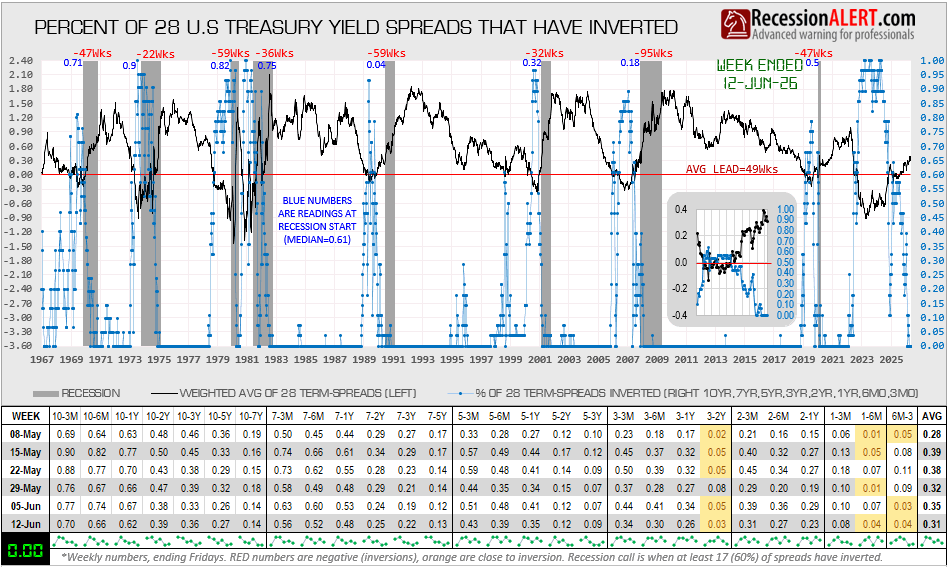
The longer the curve stays warning-free, the safer the all-clear feels. That reflex is the trap. Zero of 28 spreads inverted, the weighted average back to +0.31 and climbing — at face value, the recession watch is over. By this chart’s own history, that read is backwards. The last four recessions began at 0.04, 0.32, 0.18, and 0.50 inverted — curves that had already re-steepened. The inversion is the warning; the recession lands during the normalization that follows. We are eight weeks into that steepening, after the longest, broadest inversion the series has recorded. The clock that matters just started. The mechanism is the tell. The front end is falling because the Fed is cutting — a bull steepener, the textbook fingerprint of a central bank chasing a slowing economy, not confirming a durable expansion. Disinversion isn’t recovery; it’s the curve pricing the cuts that precede the contraction. The honest counter: this inversion already outran every prior lead — 95 weeks was the record — without a recession, so this may be the first genuine miss. Watch the long end. If steepening turns bear-led, the soft landing holds. If it stays cut-driven, the dangerous window is opening, not closing.
Market Intelligence Brief (MIB) Ver. 18.40
For professional investors only. Not investment advice.
© 2026 RecessionALERT.com
MIB Weekly: WTI -9% (Iran MoU), 2Y +9 bps (Warsh Hike Signal), SOX Record (Apple-Intel) — Which Inflation Arc Wins H2?
MIB WEEKLY DIGEST
Week of Jun 15–19, 2026
WTI crude fell 9% as the US and Iran confirmed a 60-day Hormuz ceasefire MoU (formal signing in Geneva on Friday), mechanically deflating the energy inflation premium that locked the Fed out of cuts — but Fed Chair Warsh promptly reclaimed that hawkish space: his inaugural FOMC stripped all easing bias and had 9 of 18 members projecting a 2026 hike, pushing 2Y yields to a 14-month high. Against both forces, the Philadelphia SOX hit a record — Trump’s confirmed Apple–Intel domestic foundry deal capped a week where AI hardware proved rate-cycle-agnostic. S&P +0.93% WoW, Nasdaq +2.60%, DJTA −4.25%.
TABLE OF CONTENTS
A. WEEK AT A GLANCE
B. WEEK IN MARKETS
C. WEEK’S TOP STORIES (7)
D. WEEK IN THE ECONOMY (5)
E. WEEK IN EARNINGS (1)
F. NEXT WEEK SETUP
G. CHART OF THE WEEK
A. WEEK AT A GLANCE -> TOP
The week’s dominant macro variable was the US-Iran 60-day Hormuz ceasefire MoU — confirmed Monday, formalized Wednesday — which drove WTI crude −9.1% to $76.58, mechanically deflating the energy inflation premium that had locked the Fed out of cuts for eight months. Warsh’s inaugural FOMC promptly reclaimed that hawkish space: his June 17 debut stripped all easing bias, moved the 2026 rate-median to 3.8% with 9 of 18 members projecting a hike, and pushed the 2Y yield to a 14-month high of 4.179%. Yet the S&P finished +0.93% WoW as the AI semiconductor complex — validated by the Trump-confirmed Apple–Intel domestic foundry deal and a SOX record on Thursday — proved rate-cycle-agnostic to institutional portfolios, even as NYSE Composite closed -0.41% and only 5 of 11 sectors advanced.
• S&P 500 +0.93% WoW, Nasdaq +2.60%; NYSE Composite −0.41%. Breadth was narrow: only 5 of 11 sectors advanced by week’s end; the headline S&P gain was powered by AI semiconductor concentration, not broad advance. DJTA collapsed −4.25% WoW — a Dow Theory non-confirmation — as SPCX post-IPO consolidation and defense rotation weighed on transports.
• WTI crude −9.1% WoW to $76.58 as the Strait of Hormuz began reopening under the US-Iran 60-day ceasefire; Dutch TTF −14.2% (Europe unwound more risk premium); Henry Hub +2.6% decoupled on domestic seasonality. Energy sector −5.96% WoW reversed most of its YTD +28% leadership built on the Hormuz premium.
• SOX hit a record Thursday as Trump confirmed Apple will use Intel’s IFS 18A-P process for domestic chip production. INTC +14.6% WoW; WDC +41.0% WoW (top mega-cap gainer of the week). The BofA “most crowded trade in history” designation (80% of fund managers on Tuesday) triggered a midweek −6–10% rout in the same names, which fully recovered by Thursday — the cleanest AI infrastructure crowding-risk-and-recovery sequence of 2026.
• Warsh’s FOMC June 17 dismantled the rate-cut narrative: 2Y yield +9.2 bps WoW to 4.179% (14-month high); Polymarket hike odds +11 pp to 58%; easing bias stripped; statement dramatically shortened. Retail sales +0.9% MoM (4th consecutive beat, +6.9% YoY) handed the committee full hawkish cover in a classic “good news is bad news” dynamic.
• SpaceX (SPCX) crossed $2.8T (surpassing Amazon) after a $60B all-stock acquisition of AI coding tool Anysphere (Cursor), then pulled back −10%+ intraday Thursday as options trading enabled the first institutional short-sellers on week 1 of public trading. Closed the week ~$185 — still ~37% above the $135 IPO price.
• Accenture −16–18% on guidance cut (FY26 revenue growth slashed to 3–4%): on the same day as the SOX record, AI bifurcation arrived in P&L form — hardware thrives, IT consulting implodes as AI substitution outpaces AI deal revenue scaling. IBM fell −5% sympathetically.
1. Iran as the CPI Unlock — and Its Hawkish Counterweight — WTI at $76 (down from ~$93 at peak) is deflating the energy component that drove May CPI to 4.2%; if the Geneva signing holds and Iranian barrels ramp over 4–8 weeks, the H2 2026 CPI path is fundamentally changed. But Warsh’s FOMC seized on that same potential relief to justify removing the easing bias — locking in the hawkish framework before Iran can actually deliver the disinflation. The two forces arrived in the same week and are now in structural tension over every rate-sensitive equity sector and the Fed’s September decision.
2. AI Is Rate-Cycle Agnostic — For Now — The SOX hitting a record on a hawkish FOMC week signals that institutional managers are treating AI infrastructure capex as structurally protected from rate headwinds. The Apple–Intel foundry deal and the BofA crowded-trade midweek rout both confirm the same thing from different angles: the AI trade is real but concentrated, with crowding risk (80% BofA designation, Tuesday −6–10% reversal) and structural demand (Thursday full recovery to a record) visible simultaneously. The trade survives rate shocks until it doesn’t — and the 80% “most crowded” reading historically precedes 3–6 months of sector underperformance.
3. The AI Bifurcation Has Arrived in the P&L — Accenture’s −16–18% guidance cut on the same day as the SOX record captured the week’s defining structural shift in a single session: AI hardware infrastructure (Intel, WDC, GEV) benefits; AI-displaced consulting and services (Accenture, IBM) are impaired. Enterprise clients are pausing discretionary IT projects while evaluating whether AI agents can replace the work. New bookings declining 2% at the world’s largest consulting firm is not a coincidence — it is the first P&L manifestation of a structural shift that analysts have been debating since late 2024.
B. WEEK IN MARKETS -> TOP
Two macro forces defined the week: the US-Iran 60-day ceasefire MoU — confirmed Monday, formalized Wednesday — drove WTI −9.1% as markets priced Hormuz reopening within 4–8 weeks, mechanically deflating the energy inflation premium that had locked the Fed out of cuts. Warsh immediately reclaimed that space: his inaugural June 17 FOMC stripped all easing bias, had 9 of 18 members projecting a 2026 hike, and pushed the 2Y yield to a 14-month high of 4.179%. The week’s breadth signal is the tell — S&P +0.93% but NYSE Composite −0.41%, with only 5 of 11 sectors advancing by Thursday. The AI semiconductor complex (SOX record Thursday on Apple–Intel foundry confirmation) drove the headline while Energy (−5.96%), DJTA (−4.25%), and precious metals (−7.05% silver) bore the macro repricing. The curve flattened 12.6 bps WoW: bond markets confirmed near-term hike risk but declined to endorse the long-run growth narrative.
WEEK-ON-WEEK CHANGE — Thu, Jun 18, 2026 (last trading day; Jun 19 = Juneteenth holiday):
MAJOR INDICES
The week’s key breadth tell: S&P 500 +0.93% while NYSE Composite finished −0.41% — a 1.34% gap confirming AI semiconductor leadership (Nasdaq +2.60%) drove the headline while the broad market declined. The Dow Theory signal fired: DJIA +0.71% WoW vs. DJTA −4.25% — a 4.96% divergence, more than double the 2% threshold — with transports collapsing on SPCX’s post-IPO consolidation and defense sector rotation. A transport non-confirmation of this magnitude, with NYSE Composite red, flags that the week’s gains were powered by a narrow AI hardware cohort, not a durable broad market advance.
| Index | Thu Close | WoW Change | WoW % | Why It Moved (Week) |
|---|---|---|---|---|
| S&P 500 | 7,500.65 | +69.25 | +0.93% | Iran peace deal removed Hormuz supply shock; AI semiconductor complex hit a record (Apple–Intel, Thursday); the +0.93% net masked a −1.21% Wednesday FOMC-day loss fully recovered on Thursday — a whipsaw within a net-positive week. |
| Dow Jones Industrial Avg. | 51,564.70 | +362.41 | +0.71% | Financials and Industrials led Mon–Wed on rate-hold conviction and Iran energy cost relief; Dow hit a 17th 2026 record Tuesday. IBM (−9.37% weekly) was the heaviest drag after Accenture’s guidance cut sparked IT-services sector repricing Thursday. |
| DJ Transportation Avg. | 21,637.9 | −958.8 | −4.25% | Week’s steepest major-index loss. SPCX post-IPO consolidation (fell from $201 to $185 over Mon–Thu) weighed heavily as the Industrials sector’s largest constituent. Defense rotation out (RTX −3.62%) compounded. Airline fuel-cost gains only partially offset. DJIA/DJTA gap of 4.96% WoW is the week’s sharpest Dow Theory non-confirmation. |
| Nasdaq 100 | 30,406.19 | +770.24 | +2.60% | AI semiconductor supercycle drove the outperformance: Computex 2026 (Monday), WDC/MU/MRVL upgrades (Mon–Tue), SOX record on Apple–Intel foundry deal (Thursday). Midweek BofA “crowded trade” rout (−1.89% Tuesday) fully recovered by +2.48% Thursday session. |
| Russell 2000 | 2,975.86 | +31.04 | +1.05% | Small-caps led on the final two days as FOMC certainty replaced uncertainty; Iran de-escalation supported domestic growth sentiment. RUT’s 10-session outperformance over S&P (+2.46% cumulative) signals broad market participation building beneath the large-cap AI surface. |
| NYSE Composite | 23,499.74 | −96.05 | −0.41% | Breadth was weak beneath the headline. Energy sector (−5.96% WoW) dragged the broad composite as Iran deal unwound the Hormuz premium. NYSE Composite red while Nasdaq +2.60% WoW is the week’s defining breadth signal: AI semiconductor leadership was narrow, not broad. |
VOLATILITY & TREASURIES
The curve flattened 12.6 bps WoW (39.4 → 26.8 bps, 2Y–10Y) as front-end yields jumped to 4.179% on Warsh’s inaugural FOMC — 9 of 18 members projecting a 2026 hike drove the 2Y’s +9.2 bps net move — while the 10Y eased 3.4 bps as Tuesday’s housing starts (−15.4%) created a growth-scare duration bid that survived the FOMC. VIX fell 7.3% net despite Wednesday’s intraday spike to 18.43: uncertainty resolved, not amplified. DXY crossing above 100 signals the rate-differential trade, not safe-haven capital flight — a distinction that matters for dollar direction through Q3.
| Instrument | Thu Level | WoW Change | Why It Moved (Week) |
|---|---|---|---|
| VIX | 16.40 | −1.29 (−7.29%) | Iran de-escalation removed the Hormuz geopolitical tail risk; Warsh FOMC initially spiked VIX to 18.43 Wednesday but Thursday’s Apple–Intel catalyst resolved the uncertainty. Net-week VIX decline: geopolitical premium removed (bullish) outweighed rate-hike signal (bearish). |
| 10-Year Treasury Yield | 4.447% | −3.4 bps | Modest yield decline despite hawkish FOMC — housing starts −15.4% Tuesday created a growth-scare duration bid; 20-year auction drew 73.2% foreign demand (vs 64.9% average). Bond market declined to confirm the FOMC’s near-term hawkishness at the long end. |
| 2-Year Treasury Yield | 4.179% | +9.2 bps | Sharpest WoW curve move. Warsh’s debut FOMC (June 17) stripped easing bias and moved the dot-plot median to 3.8% with a majority-hike signal; retail sales +0.9% (4th consecutive beat, +6.9% YoY) and import prices at 6.7% YoY provided the data cover for the repricing. |
| US Dollar Index (DXY) | 100.82 | +1.04 (+1.04%) | Dollar strengthened on Warsh’s hawkish FOMC signal — higher US rates vs. global peers drew carry-trade flows; DXY crossed above 100 for the first time this week. Iran de-escalation (normally dollar-softening on risk-on) was offset by the rate-differential widening thesis. |
COMMODITIES
Gold’s −0.18% net week conceals a violent intra-week round trip: Iranian peace news drove it to $4,353 mid-week, then the Warsh FOMC + MoU execution simultaneously removed two distinct premiums (rate-hedge appeal and geopolitical safe-haven) in a single Thursday session, erasing the gain. Silver’s −3.34% underperformance vs. gold reveals the dual-premium mechanics most clearly — the industrial safe-haven overlap amplified the Thursday selloff more than pure monetary gold. Bitcoin’s −0.91% tracking DXY strength (not the SOX record) confirmed it functioned as a dollar-inverse asset this week, not an AI-narrative proxy.
| Asset | Thu Price | WoW Change | WoW % | Why It Moved (Week) |
|---|---|---|---|---|
| Gold | $4,227.75/oz | −$7.67 | −0.18% | Net week near-flat masks a round trip to $4,353 mid-week then a −3.51% Thursday collapse. Warsh’s hawkish FOMC + Iran MoU execution simultaneously removed the rate-hedge bid and geopolitical safe-haven premium in a single session. |
| Silver | $65.778/oz | −$2.272 | −3.34% | Sharper than gold due to silver’s dual monetary/industrial role; hit $70+ mid-week then −7.05% Thursday as geopolitical and monetary premiums simultaneously unwound. The industrial-safe-haven overlap amplified the Thursday move. |
| Copper | $6.3780/lb | −$0.1003 | −1.55% | DXY +1.04% WoW outweighed AI/electrification demand optimism. Iran de-escalation was expected to boost industrial copper demand (supply chains normalizing) but dollar strength dominated. Modest decline consistent with mixed growth signals. |
| Platinum | $1,696.40/oz | −$22.40 | −1.30% | Precious metals complex decline on hawkish Fed and Iran MoU execution; −5.38% Thursday (largest precious metals decliner) as auto-catalyst and industrial demand concerns compounded the monetary repricing. |
| Bitcoin | $62,906 | −$578 | −0.91% | Tracked DXY strength rather than the AI-driven equity risk-on tape. Decoupled from the SOX record — BTC functioned as a dollar-inverse asset, not an AI-narrative proxy. No crypto-specific catalyst all week. |
ENERGY
The US-Iran 60-day ceasefire MoU drove WTI’s 9.1% WoW decline as markets priced Hormuz-transiting Iranian barrels returning within 4–8 weeks. Dutch TTF fell 14.2% WoW versus WTI’s 9.1% — Europe had more geopolitical premium to unwind; Henry Hub gained 2.6% independently on seasonal US demand. Oil declining while equities gained (+0.93% S&P WoW) is the demand-neutral supply-normalization read: the Hormuz risk premium was removed, not a growth scare. The EIA’s 10th consecutive crude draw — US commercial stocks at a 40-year low — provided a near-term floor that prevented a larger rout.
| Asset | Thu Price | WoW Change | WoW % | Why It Moved (Week) |
|---|---|---|---|---|
| Crude Oil (WTI) | $76.58/bbl | −$7.66 | −9.09% | US-Iran 60-day ceasefire MoU (confirmed Monday, formalized Wednesday) removed the Hormuz geopolitical supply premium embedded since April. WTI fell from $84.24 to $76.58 over 4 sessions; EIA’s 10th consecutive crude draw (−8.26M bbls, 40-year inventory low) provided a near-term floor. |
| Crude Oil (Brent) | $79.38/bbl | −$7.38 | −8.50% | Same Iran supply normalization driver. Tight WTI-Brent spread ($2.80 at week end) confirms a global supply story, not a regional disruption. Dutch TTF −14.2% WoW — Europe priced out more geopolitical premium than US crude markets. |
| Natural Gas (Henry Hub) | $3.217/MMBtu | +$0.082 | +2.62% | Decoupled entirely from crude all week — domestic US gas supply/demand is weather-driven and LNG-export-driven, indifferent to the Strait of Hormuz. Summer cooling demand and LNG export demand provided independent support throughout the week. |
| Natural Gas (Dutch TTF) | $13.61/MMBtu | −$2.26 | −14.24% | Europe aggressively priced out the Iran/Middle East supply risk premium across the week. Iranian LNG and pipeline flows expected to return in 4–8 weeks; week’s largest WoW percentage decline in the B1 table. |
S&P 500 SECTORS — WEEKLY ROTATION
Technology and Industrials led all 11 sectors this week — but both moves were single-cluster-driven, not broad. Four of the week’s top-5 gainers (WDC +41%, INTC +15%, SNDK +16%, STX +23%) are Technology names: strip them out and Tech’s +3.95% shrinks toward negligible. GEV alone (+22% weekly) drove a large share of Industrials’ +4.59% gain. Energy’s structural laggard signal deepened: worst sector across 1W (−5.96%), 1M (−11.94%), AND 3M (−9.25%) simultaneously — the Iran deal systematically extracting the Hormuz premium that powered its +28% YTD leadership through April. Broad-based sector leadership this was not: five sectors declined WoW, and the breadth verdict favors caution despite the headline indices.
| Sector | 1-Week | 1-Month | 3-Month | 6-Month | YTD | 12-Month |
|---|---|---|---|---|---|---|
| Industrials | +4.59% | +9.26% | +13.71% | +20.53% | +20.92% | +33.62% |
| Technology | +3.95% | +7.75% | +30.74% | +26.48% | +24.77% | +47.72% |
| Financial | +2.24% | +5.78% | +12.08% | +2.25% | +1.54% | +15.70% |
| Basic Materials | +1.77% | +3.35% | +9.20% | +16.16% | +14.37% | +41.99% |
| Utilities | +1.08% | +0.04% | −3.63% | +4.24% | +4.48% | +13.71% |
| Communication Services | +0.93% | −4.55% | +6.60% | +3.13% | +1.86% | +24.93% |
| Consumer Cyclical | +0.44% | −0.03% | +6.34% | −5.25% | −4.03% | +8.04% |
| Consumer Defensive | −2.21% | −5.21% | +0.93% | +4.58% | +6.28% | +5.01% |
| Real Estate | −2.23% | +0.07% | +4.49% | +7.04% | +7.30% | +6.15% |
| Healthcare | −2.28% | +1.61% | +2.71% | −2.09% | −2.66% | +12.91% |
| Energy | −5.96% | −11.94% | −9.25% | +23.48% | +20.00% | +22.20% |
TOP WEEKLY MOVERS:
All five weekly gainers share a single theme: the AI supply chain from silicon (INTC +14.6%) to memory (WDC +41%, SNDK +16%, STX +23%) to power infrastructure (GEV +22%) — the week’s leaderboard is an end-to-end slice of the AI buildout thesis. Multi-year momentum across every gainer (SNDK +4,586% Year, WDC +1,161%, STX +715% per the underlying screener) confirms regime-leadership moves, not counter-trend bounces — yet the Tuesday −6% to −10% single-session reversal across the same names (on BofA’s “most crowded trade” designation) proved the crowding risk is real. The decliners were split: Energy names (CVX, XOM) on Iran deal supply normalization, and AI-disruption losers (IBM) on Accenture’s consulting guidance cut revealing the services-layer impairment in the P&L for the first time.
TOP 5 WEEKLY GAINERS
| Ticker | Week | YTD | Year | Why It Moved |
|---|---|---|---|---|
| WDC | +40.99% | +333.17% | +1160.74% | Computex 2026 AI storage showcase (Ultrastar Data 3000 JBODs); JPMorgan raised PT to $650; Morgan Stanley upgrade projecting HDD demand growing 40–50%/yr vs. 30–35% supply through 2028, raising 2028 EPS estimates 70% above consensus. Sixth consecutive day of gains by Thursday. Structural supply deficit is the thesis, not near-term momentum. |
| STX | +23.29% | +288.62% | +715.10% | Correlated with WDC on AI storage infrastructure bottleneck thesis; Computex 2026 AI storage demand wave; Morgan Stanley bullish note on HDD structural demand deficit. Dividend announcement ($0.74, ex-date June 24) provided an additional catalyst. YTD +289% confirms regime leadership, not a bounce. |
| GEV | +22.38% | +69.80% | +126.39% | Bernstein SocGen initiated with Outperform, citing record backlogs and AI data center electricity demand (AI’s primary bottleneck has shifted from chips to power). US-Iran MoU also positive: the deal supports large-scale capital investment in GEV’s gas power, grid electrification, and wind turbine businesses. EPS estimates revised +72.92% for 2026. |
| SNDK | +16.12% | +820.36% | +4586.29% | Thursday surge on Trump’s Apple–Intel foundry announcement (broad semiconductor complex rerate); Morgan Stanley raised SNDK earnings estimates on AI memory upcycle; Apple’s pricing signal confirming rising memory costs validated the structural demand thesis. SNDK’s +4,586% Year gain makes this momentum continuation, not reversal. |
| INTC | +14.56% | +263.12% | +523.50% | Triple catalyst: BofA double upgrade (Underperform to Buy, prior week, $135 PT, $170B server CPU TAM by 2030) carried momentum into the week; Thursday’s Trump Truth Social confirmation that Apple will use Intel’s IFS 18A-P process for domestic chip production drove +10.6% on the day alone; Intel named new EVP of Intel Foundry on the same day. Historic foundry thesis validation. |
TOP 5 WEEKLY DECLINERS
| Ticker | Week | YTD | Year | Why It Moved |
|---|---|---|---|---|
| IBM | −9.37% | −15.90% | −12.04% | Accenture’s −16–18% guidance cut (FY26 revenue growth slashed to 3–4%, new bookings −2%) triggered IT-services sector selloff Thursday; IBM separately released a study showing 91% of enterprise execs lack full visibility into their AI dependencies. IBM Consulting grew just 1% in Q1 2026 — the structural AI-substitution threat to the services layer arrived in P&L form. IBM YTD −15.90% = structural underperformer, not a bounce candidate. |
| CVX | −6.56% | +13.92% | +17.17% | US-Iran peace deal collapsed the Hormuz geopolitical risk premium that drove Energy’s YTD +28% leadership. WTI fell from $84 to $76 over 4 sessions as Iran oil sanctions waiver and Hormuz reopening were formalized. Jefferies Buy rating on June 15 could not overcome the macro oil price decline. CVX’s YTD +13.92% suggests longer-term holders are still profitable — but the near-term oil path is structurally bearish. |
| XOM | −6.00% | +14.52% | +21.75% | Same Iran supply normalization driver as CVX. US-Iran interim agreement signed June 17, with first tanker re-transits underway by Thursday. BofA upgraded XOM to Buy June 15 (Neutral previously) — positive catalyst insufficient to offset the structural oil price decline thesis as Iranian barrels approach market return. |
| MRK | −5.71% | +8.18% | +43.61% | CMS proposed locking in lower prices in Medicare drug price negotiation program (June 15); ex-dividend date June 15 (natural selling around dividend capture); Healthcare sector rotation out as Iran deal reduced defensive positioning. Capvaxive FDA additional indication approval was positive but insufficient to offset pharma-pricing headwinds. |
| LLY | −5.37% | +2.22% | +39.94% | Profit-taking after strong 12.5% 1-month run; Novo Nordisk sought China approval for Wegovy pill on June 15 (intensifying GLP-1 rivalry); same Medicare drug pricing headwinds as MRK; acquired 4E Therapeutics (June 16). Rotation away from defensive dividend-payers as Iran deal reduced the geopolitical safe-haven bid in healthcare names. |
C. WEEK’S TOP STORIES -> TOP
Three threads shaped the week. The geopolitical arc (#1) transformed the US-Iran Hormuz standoff into a formalized 60-day ceasefire — WTI’s −9% WoW is the CPI variable of 2026 now in motion. The monetary arc (#2) arrived the same week: Warsh’s debut FOMC dismantled the rate-cut thesis that anchored 2025 equity valuations in a single press conference. Both arcs pull on the same inflation variable in opposite directions — the tension between them defines the H2 outlook. The AI arc (#3, #4, #6, #7) ran on its own logic: hardware validated at a SOX record, consulting impaired, SpaceX revalued its entire business model in week one.
UNCERTAIN
1. US-Iran Peace Deal: From Draft MoU to 60-Day Hormuz Ceasefire — WTI −9% to $76.58 This Week; Geneva Signing Scheduled for Juneteenth (June 19)
The core facts:The US-Iran peace framework evolved through three distinct stages across four trading days. Monday (Jun 15): Washington, Tehran, and Pakistani negotiators confirmed a Memorandum of Understanding signing set for Friday in Switzerland; WTI fell 4.2% to $81.32 as markets priced out the Hormuz supply premium. Wednesday (Jun 17): The 60-day ceasefire MoU was formally signed — key terms: removal of US naval blockade of Iranian ports, resumption of Iranian crude exports immediately, oil sanctions waived (not eliminated), Strait of Hormuz opened to toll-free transit. First tankers began re-transiting the Strait by Thursday. WTI fell another 5% to ~$75, settling the week at $76.58 vs. $84.24 last Friday (−9.1% WoW). Thursday (Jun 18): The EIA reported the 10th consecutive weekly crude draw (−8.26M barrels); US commercial crude stocks at a 40-year low — providing a near-term price floor. The IEA’s June Oil Market Report projected a 5 mb/d global supply surplus in 2027 as Iranian barrels return. A formal Geneva signing ceremony was scheduled for Friday June 19 — a US market holiday (Juneteenth) — with follow-on nuclear talks to begin immediately after.
Why it matters:The Hormuz risk premium has been the primary driver of elevated oil prices and the inflation overhang that locked the Fed out of cuts in 2026. The energy component rose +23.5% YoY and drove May CPI to 4.2%. WTI at $76 with a credible path to $70–73 (if the IEA’s 2027 supply-surplus projection materializes) changes the H2 CPI arithmetic: if June and July prints land near 3.0–3.5% on energy normalization, the case for rate hikes weakens and the easing debate reopens. The UNCERTAIN classification reflects two layers: (1) the Geneva signing is still the risk event for this weekend — any breakdown immediately reverses WTI, energy sector, defense stocks, and precious metals; (2) the MoU is a 60-day bridging framework, not a permanent peace agreement. Iran’s crude ramp takes 4–8 weeks to reach global markets, meaning the supply relief is weeks away even if the signing holds. The IEA’s 2027 surplus projection (+8 mb/d supply surge) is the structural ceiling on energy sector valuations regardless of near-term oil prices.
What to watch:Geneva signing outcome — this weekend’s critical binary (success = Iran energy trade continues; breakdown = WTI spike, energy/defense/gold reverse). First Iranian crude export manifests (4–8 weeks). EIA weekly crude inventory (June 24) for first signal of whether Iranian supply is reaching US markets. OPEC+ production response as the Saudi-led counterbalance. June CPI (mid-July) as the first quantified test of the energy disinflation thesis.
BEARISH
2. Warsh’s Debut FOMC Dismantles the Rate-Cut Thesis: 9 of 18 Members Project 2026 Hike; Easing Bias Stripped; 2Y Yield Hits 14-Month High of 4.179%
The core facts:Tuesday (Jun 16): Warsh’s inaugural two-day FOMC meeting opened. Pre-meeting data was already hawkish: housing starts −15.4% to 1.177M (weakest since May 2020, 18% miss vs. consensus) and import prices +6.7% YoY (highest since August 2022) arrived simultaneously. Wednesday (Jun 17): May retail sales printed +0.9% MoM (4th consecutive beat, +6.9% YoY) hours before the decision, handing the committee full hawkish cover. The FOMC voted 12-0 to hold rates at 3.50–3.75% but stripped all easing bias from the statement — a dramatically shortened policy release. The dot plot shifted: 9 of 18 members projected at least one 2026 hike; median year-end 2026 FFR moved to 3.8% from 3.4% in March. Warsh did not submit his own dot projection, and signaled fewer future press conferences. 2Y Treasury yield surged +15 bps to 4.21% on the day; VIX +12.31%; S&P −1.21%, Dow −507 pts. Polymarket: hike probability 37% → 58% (post-FOMC); cut probability 30.2% → 18.5%. Thursday (Jun 18): Philly Fed Prices Paid surged to 53.2 (from 47.9), providing a second consecutive hawkish data point. Markets absorbed the FOMC shock by Thursday’s close: S&P recovered +1.09% as Apple–Intel and AI hardware decoupled from rate anxiety.
Why it matters:Warsh’s debut resets the 2026 monetary policy framework entirely. Markets entered the week pricing some probability of rate cuts; they exited pricing a potential hike. The removal of easing bias — combined with 9 of 18 members projecting a hike — marks a structural break from the prior rate-cutting narrative that underpinned 2025’s equity expansion and early 2026’s valuations. Warsh’s communication overhaul (fewer press conferences, compressed statement) structurally increases policy uncertainty for the rest of the year — future meetings will carry higher surprise risk. For equity portfolios: this removes the rate-cut catalyst that anchored growth-equity valuations in 2025 and raises the discount rate for all long-duration assets. Rate-sensitive sectors (REITs, utilities, homebuilders, high-multiple tech) face systematic repricing. The session’s breadth signal confirmed markets read this as rate-fear, not recession fear: VIX +12.31% but no safe-haven gold bid (gold −1.68%); 2Y surged while 10Y only rose 6 bps — front-loaded hike pricing, not long-run growth deterioration. The market’s fast recovery Thursday (S&P +1.09%) on Apple–Intel confirms that AI infrastructure is treated as rate-cycle-agnostic, even as rate-sensitive sectors remain pressured.
What to watch:September FOMC as the earliest plausible hike window — CME FedWatch hike odds for September as real-time calibration. June NFP (July 3) as the first major post-FOMC labor market test. June PCE (late June) — the data that will determine whether September is live or academic. Warsh public speeches for signals on how he operationalizes “fewer press conferences.”
BULLISH
3. AI Semiconductor Supercycle: Computex Drives PHLX +7.9% (Mon), BofA “Most Crowded Trade in History” Triggers −6–10% Rout (Tue), Apple–Intel Foundry Confirmation Sets SOX Record (Thu)
The core facts:Monday (Jun 15): Computex 2026 ignited the week: WDC +16.1% to $653.53 (JPMorgan PT raised to $650); MU +10.9%; MRVL +10.4%; PHLX Semiconductor Index (SOX) +7.9% — its largest single-session gain since April 2025. Key announcements: Micron’s HBM4 sold out through year-end; NVIDIA–SK Hynix multi-year supply cooperation signed; Western Digital showcased Ultrastar Data 3000 JBODs; Morgan Stanley upgraded WDC projecting HDD demand growing 40–50%/yr vs. 30–35% supply through 2028 (2028 EPS est. raised 70% above consensus). Tuesday (Jun 16): Bank of America’s June fund manager survey revealed 80% of respondents classify semiconductors as “the most crowded trade in history.” MRVL −9.78%, INTC −8.45%, KLAC −7.44%, AMD −7.30%, MU −6.18%; Technology sector −2.52%. Wednesday (Jun 17): AI hardware decoupled from the FOMC selloff — AVGO +4.30%, AMAT +4.35%, MRVL +3.90%, WDC +4.56% against a −1.21% S&P tape. Thursday (Jun 18): President Trump confirmed on Truth Social that Apple has agreed to work with Intel to design and manufacture chips domestically using Intel’s 18A-P process node (MacBook M7 SoC target, mass manufacturing late 2027). SOX surged 6% to a record high. INTC +10.6%, SNDK +11.5%, MU +8.7%, KLAC +8.7%, MRVL +7.3%.
Why it matters:The week’s intra-week volatility pattern — SOX +7.9% Monday, −6–10% Tuesday, recovery Wednesday, SOX record Thursday — is the most analytically revealing semiconductor week of 2026. The BofA “most crowded trade” designation (80% of fund managers) is historically a 3–6 month underperformance precursor. Yet the Thursday Apple–Intel catalyst drove a full recovery to a record, confirming that structural earnings growth visibility can override crowding risk in the near term. Apple as the world’s most demanding chip customer committing to Intel’s IFS validates the US domestic semiconductor reshoring thesis at a scale that no government contract or analyst note could provide: the company that built its supply chain advantage on TSMC’s Taiwan fabs is now committing to domestic production. The SOX at a record on a hawkish FOMC week confirms institutional managers are treating AI infrastructure capex as rate-cycle-agnostic — demanding, not cyclical. WDC’s +41% WoW and INTC’s +14.6% WoW are the week’s top two mega-cap performances (see B4 Sector rotation table).
What to watch:Intel’s 18A-P yield milestones as the critical execution risk — Apple’s shift to IFS only scales if Intel achieves competitive yields. Nasdaq-100 SPCX inclusion timing as the next passive-buying trigger. Micron Q3 FY2026 earnings (late June) — the first quantification of HBM4 demand in reported revenue. Apple formal confirmation of Intel deal scope (not yet issued as of Thursday).
UNCERTAIN
4. SpaceX (SPCX): Day 2 +19% to $2.8T (Passes Amazon); $60B All-Stock Cursor AI Acquisition; Options Unlock Enables First Institutional Shorts; Correction to ~$185
The core facts:Monday (Jun 15): SPCX +19.6% Day 2 to $192.46 — market cap crossed $2.5T, surpassing Apple as world’s largest public company. Elon Musk publicly projected $1 trillion in SpaceX annual revenue by 2030. Tuesday (Jun 16): SpaceX filed an SEC Form 8-K announcing a definitive agreement to acquire Anysphere Inc. — developer of Cursor, the leading AI-powered coding tool — in a $60 billion all-stock transaction. SPCX valuation crossed $2.8T, surpassing Amazon as the 5th-largest US public company. Options on SPCX began trading Wednesday. Thursday (Jun 18): SPCX fell as much as −10.3% intraday — the first session where institutional bears could use options to short the stock. IPO prospectus disclosures drew scrutiny: $4.9B net loss in 2025, $4.28B net loss in Q1 2026 alone, with Starlink the only profitable segment. SPCX closed the week approximately $185 — ~37% above the $135 IPO price but down materially from the $201 intraday high on Tuesday. (See also: B4 Gainers — SPCX was not in the top-5 gainers this week, which only covers names that gained WoW; SPCX ended the week below Monday’s open.)
Why it matters:A $60B acquisition in week 1 of public trading is unprecedented and reveals a strategic pivot that was not in the IPO thesis: SpaceX is using its newly minted public equity as acquisition currency to enter AI developer software (Cursor) alongside its hardware infrastructure (rockets, Starlink). This broadens the SpaceX thesis dramatically but adds execution risk — integrating Cursor’s AI coding platform into SpaceX’s engineering stack requires a product strategy that hasn’t yet been explained publicly. Options unlocking restored the two-sided market: without options in days 1–2, institutional bears could not participate in price discovery, allowing momentum buyers to push prices toward $201. At $2.8T valuation with $9B+ in annual losses, SPCX prices extraordinary future profitability from Starlink global satellite expansion and Starship heavy-lift commercialization — timelines measured in years. The UNCERTAIN classification reflects the binary nature of this week: still ~37% above IPO price but with $60B acquisition risk, options-enabled downside discovery, and no precedent for a company at this valuation scale with this loss rate going public.
What to watch:Nasdaq-100 inclusion announcement (expected within weeks per Nasdaq’s rewritten eligibility criteria) — this passive buying trigger will compress the float against institutional demand. DOJ antitrust review of the Cursor acquisition. SPCX sustaining above $135 IPO price as the institutional confidence threshold. Starlink subscriber growth and monthly ARPU as the first fundamental anchor for the $1T revenue projection.
BEARISH
5. Housing Structural Contraction Deepens: NAHB 35 (26th Sub-50 Month), May Starts −15.4% to 1.177M (Weakest Since May 2020); Pending Sales +3.8% Creates Demand/Supply Split
The core facts:Monday (Jun 15): NAHB June Housing Market Index came in at 35 — the 26th consecutive month below 50, the longest sustained contraction in the index’s modern history. 35% of builders cutting prices (up from 32%); buyer traffic at 25 (near historic lows); mortgage rates at 6.6%. Tuesday (Jun 16): Housing Starts collapsed −15.4% MoM to 1.177M SAAR — the weakest reading since May 2020, 18% below the 1.430M consensus. Building Permits were relatively stable at 1.413M (−0.7%), creating a sharp starts/permits divergence. The Atlanta Fed GDPNow revised Q2 2026 growth down to 2.8% from 3.3% on the data. Wednesday (Jun 17): Pending Home Sales +3.8% MoM vs. 0.8% expected — nearly 5x the consensus — across all four US census regions. NAR cited “pent-up demand” and consumer acceptance of 6%+ mortgage rates. Thursday (Jun 18): Freddie Mac 30-year mortgage rate fell to 6.47% (1-month low) as the Iran deal’s energy-price relief reduced the inflation premium embedded in Treasury yields.
Why it matters:The starts collapse (−15.4%) vs. permits near-flat (−0.7%) creates the most important housing market split of the cycle: buyers want to transact (pending sales +3.8%) but builders are stopping construction. This is structurally bullish for home prices (demand present, supply contracting) but bearish for the economy (residential investment is a direct GDP component — the GDPNow revision to 2.8% captures this). The Warsh FOMC’s hawkish pivot Wednesday could push mortgage rates back toward 6.75–7.0%, potentially capping the pending-sales recovery before it converts to closings — a classic monetary policy transmission risk. The 26-month continuous sub-50 NAHB reading (the longest in modern history) represents a structural demand suppression that is not self-correcting at current rates. Iran deal energy relief (30-year mortgage down to 6.47%) is the counterforce, but it depends entirely on the Geneva signing holding.
What to watch:June Housing Starts (mid-July) — can the permits-starts divergence close as mortgage rates ease? 30-year mortgage rate trajectory post-Geneva signing. Homebuilder Q2 2026 earnings calls (July) for cancellation rates, new order volumes, and guidance on whether the NAHB sub-50 streak is ending.
BEARISH
6. Accenture −16–18%: AI Bifurcation Arrives in the P&L — FY26 Revenue Growth Cut to 3–4%, New Bookings −2%; IBM −5% Sympathetically on the Same Day as the SOX Record
The core facts:Thursday (Jun 18): Accenture (ACN) reported fiscal Q3 2026 results: EPS beat ($3.80 actual vs. $3.71 estimate) but cut full-year revenue growth guidance to 3–4% (from 3–5%); Q4 revenue guidance $17.75–18.4B vs. $18.47B consensus. New bookings declined 2% for the quarter ended May 31 — the leading signal that the consulting pipeline is contracting. Reasons: AI disruption compressing consulting model, cautious enterprise IT spending, material drag from US federal government business. ACN fell 16–18% — worst single-day decline in years. IBM fell ~5% sympathetically. Note: ACN is Irish-domiciled at ~$78B market cap (below the Earnings Watch $100B threshold; covered here for its sector-level market signal). The announcement occurred on the same Thursday when the SOX hit a record high on the Apple–Intel foundry deal — hardware and consulting diverged in the P&L simultaneously.
Why it matters:New bookings declining 2% at Accenture is the forward signal that matters: enterprise clients are pausing or reducing discretionary IT consulting projects while evaluating whether AI agents can perform that work at lower cost. AI deal announcements are increasing, but AI deal revenue has not yet scaled to replace the traditional consulting revenue that AI is simultaneously cannibalizing. The Accenture print on the day of the SOX record captures the week’s defining structural dynamic in one session: AI hardware infrastructure (silicon, memory, power) is in a demand boom; the human services layer built on top of IT systems is in early-stage structural compression. IBM’s −5% sympathetic move confirms the market reads this as sector-wide — Infosys, Wipro, Cognizant, Oracle consulting, and SAP professional services all face the same model risk. IBM separately released a study showing 91% of enterprise executives do not fully understand their AI dependencies — the very opacity driving clients to evaluate AI substitution rather than commit to consulting engagements.
What to watch:IBM Q2 2026 earnings (late July) for the first direct evidence of consulting revenue compression at scale. Oracle and SAP professional services guidance updates. Salesforce, ServiceNow Q2 earnings — where AI substitution risk for seat-based software compounds the consulting threat. Accenture’s Q4 FY2026 new bookings (next report) as the leading indicator of whether the pipeline stabilizes.
BEARISH
7. Meta −5.44%: AI Head of Product Departs a Freshly Created Role; School Addiction Trial Strips Section 230 Design Protections; $145B CapEx Overhang Compounds Risk
The core facts:Wednesday (Jun 17): Reuters reported that Emily Dalton Smith — Meta’s Head of AI Product for its “AI for Work” transformation initiative, appointed approximately two months earlier as part of a company-wide AI reorganization — is leaving Meta. The departure from a freshly created role at the center of Meta’s highest-priority AI execution track is the primary catalyst. META fell −5.44% — worst single-day mega-cap decliner of the week. Background: the federal multidistrict school addiction bellwether trial commenced June 15, with design defect claims having stripped Section 230 liability protections for algorithmic recommendation systems. Meta’s 2026 CapEx guidance: $125–145B. Thursday (Jun 18): Meta separately secured AI computing agreements with Crusoe — advancing AI infrastructure buildout independent of product leadership questions.
Why it matters:Emily Dalton Smith’s departure from a freshly appointed role is characteristic of either a strategic pivot or management friction at the most critical point of Meta’s AI transformation — precisely when execution of the $145B capex thesis needs to begin delivering AI-agent product revenue. Losing the product lead on AI-agent capabilities at this stage raises the question: is the strategy intact, or is there internal disagreement about execution approach? This is not a routine executive transition. The school addiction trial creates a separate open-ended legal liability: if design defect claims succeed in this bellwether case, Meta’s platform architecture faces injunctive risk beyond financial penalties — potentially forcing redesigns of core algorithmic recommendation systems that drive advertising revenue. The combination — AI product leadership gap, $145B capex commitment without near-term AI revenue justification, and legal liability — creates a multi-front headwind entering Q2 earnings season. The Crusoe computing deal (Thursday) confirms AI infrastructure execution is proceeding independently, but the product layer is the unresolved risk.
What to watch:Meta’s replacement appointment for Head of AI Product — timing and seniority as a signal of organizational health. Q2 2026 earnings (late July) for first AI-agent product revenue metrics and CapEx guidance confirmation. School addiction trial jury verdict or settlement as the legal liability quantification event. Any court injunction seeking to alter Meta’s algorithmic recommendation systems prior to trial conclusion.
D. WEEK IN THE ECONOMY -> TOP
A stagflation pulse defined the week’s data: import prices hit 6.7% YoY — highest since August 2022, with tariff cost-push spreading beyond fuel into capital goods — on the same week housing starts plunged −15.4% to a 6-year low. The Fed answered with a decisive framework reset: Warsh’s debut FOMC stripped all easing bias and had 9 of 18 members projecting a 2026 hike, pushing Polymarket hike odds from 47% to 58% WoW while 2Y yields rose 9.2 bps to a 14-month high (see Vol & Treasuries table in Section B). Simultaneously, the Iran deal’s disinflation impulse (WTI −9% WoW; energy sector −5.96%) reopened cut probability from ~3% to 18.5% — the two forces produced the most complex dual-signal week of 2026. Tuesday’s S&P Global Flash Manufacturing PMI will determine whether Philly Fed’s Prices Paid spike at 53.2 was regional noise or the national factory-gate re-acceleration that would lock in the September hike case.
POLYMARKET ODDS — WEEK-ON-WEEK SHIFT:
| Market | Last Friday (Jun 12) | This Thursday (Jun 18) | Δ |
|---|---|---|---|
| US Recession by end-2026 | ~19% | 13% | −6 pp |
| Fed rate hike in 2026 | 47% | 58% | +11 pp |
| Fed rate cuts ≥1 in 2026 | ~3% | 18.5% | +15.5 pp |
Note: This week’s Polymarket odds reflect competing forces. The Iran deal (oil −9% WoW) reopened cut probability from near-zero to 18.5%; Warsh’s hawkish FOMC simultaneously drove hike odds to 58%. The net result is the most complex dual-signal Polymarket week of 2026: recession odds declined (BULLISH), hike odds rose (BEARISH), and cut odds rose from near-zero on Iran disinflation (BULLISH for rate-sensitives long-term). Thursday’s odds; Jun 19 was Juneteenth — markets closed.
UNCERTAIN
1. Retail Sales +0.9% MoM in May — 4th Consecutive Beat, +6.9% YoY; GDPNow Revised to 3.0%; “Good News Is Bad News” as Strong Consumer Handed Warsh Hawkish Cover (Census Bureau, Wed Jun 17)
What they’re saying:Advance retail sales May +0.9% MoM (vs. +0.5% expected) — the 4th consecutive monthly beat. Control group (the cleanest GDP proxy) +0.7% vs. +0.4% consensus. YoY growth: +6.9%, fastest since Q4 2022. Atlanta Fed GDPNow revised to 3.0% from 2.8% (Tuesday’s housing starts had cut it to 2.8% the prior day — consumer spending reversed it within 24 hours). The data arrived at 8:30am ET — hours before the 2:00pm FOMC decision.
The context:The 4th consecutive beat at +6.9% YoY is structurally incompatible with rate cuts when PCE sits at 4.2%. Consumer spending at this pace gave the FOMC committee all the data justification needed to strip easing bias and shift the dot plot toward hikes. This is the “good news is bad news” dynamic formalized: strong demand = Fed justified in tightening = equity multiple compression. The initial equity rally on the strong print (+0.5% before noon) reversed to −1.21% after the FOMC decision. The 4-quarter streak of beats also undermines any soft-landing narrative that requires consumption moderation to bring inflation down — consumers appear structurally unaware of the policy tightening that is needed to stop them.
What to watch:June retail sales (July 15) — a 5th consecutive beat would eliminate any remaining dovish argument heading into the September FOMC. June PCE (late June) as the first post-FOMC consumer spending read. Whether Iran-related energy price relief translates into real spending increase or just nominal stabilization.
BEARISH
2. May Housing Starts −15.4% to 1.177M SAAR (Weakest Since May 2020), 18% Miss; NAHB June 35 (26th Sub-50); Pending Sales +3.8% Reveals Demand/Supply Split (Census Bureau / NAHB / NAR, Mon–Wed)
What they’re saying:NAHB June HMI: 35 (prior 37, cons. 36) — 26th consecutive month below 50; 35% of builders cutting prices (up from 32%); traffic 25. Housing Starts: 1.177M SAAR May (−15.4% MoM, −8.7% YoY, 18% miss vs. 1.430M consensus) — weakest since May 2020. Building permits 1.413M (−0.7%, near-flat). GDPNow cut to 2.8% (reversed same day by retail sales). Pending Home Sales: +3.8% MoM (vs. 0.8% cons.) — all four regions positive; NAR cited pent-up demand and 6%+ rate acceptance. 30-year mortgage: 6.47% (Thursday, 1-month low) on Iran deal inflation relief.
The context:The permits-starts divergence (permits −0.7%, starts −15.4%) is the key analytical signal: builders aren’t cancelling plans, they’re delaying groundbreakings — a “wait-and-see” posture that could reverse if mortgage rates continue declining. The demand/supply split is bearish for the macro but creates housing price persistence: buyers want to transact (pending sales +3.8%) but supply is contracting sharply. The Warsh hawkish FOMC Wednesday competes directly with the Iran deal’s mortgage-rate relief: if the hike signal pushes 30-year rates back toward 6.75–7.0%, the pending-sales recovery caps before converting to closings.
What to watch:June Housing Starts (mid-July) for whether the permit-starts gap closes. 30-year mortgage rate post-Geneva signing. Homebuilder Q2 earnings (July) for cancellation rates and forward order volumes.
BEARISH
3. May Import Prices +1.9% MoM vs. +1.0% Expected; YoY Surges to 6.7% — Highest Since August 2022; Tariff Cost-Push Broadening Beyond Fuel into Capital Goods (BLS, Tue Jun 16)
What they’re saying:May import prices +1.9% MoM (nearly double the +1.0% consensus). YoY +6.7% — highest since August 2022. Breakdown: fuel import prices +12.5% MoM; nonfuel +0.8%; capital goods +1.3%. Export prices +1.3% MoM; YoY +11.2%. Data arrived alongside Tuesday’s housing starts catastrophe.
The context:The nonfuel (+0.8% MoM) and capital goods (+1.3% MoM) acceleration is the structural concern: tariff cost-push is broadening beyond the Iran energy shock into durable goods and business equipment. This is the two-track inflation problem — Iran deal reduces the energy CPI component, but tariff-driven goods inflation keeps building independently. Capital goods at +1.3% MoM signals that business investment costs are rising, compressing corporate margins on top-line growth. The data arrived on FOMC Day 1 and all but locked in Warsh’s hawkish dot-plot the following morning. For June CPI: the pipeline from import prices to consumer prices runs 1–3 months, meaning July CPI could reflect May’s import price surge even if June energy prices fall further.
What to watch:July CPI (mid-July) for import price pass-through to consumer goods. Any tariff de-escalation announcement with Vietnam, Bangladesh, Cambodia — the primary sources of nonfuel import price acceleration. June PPI (mid-July) as the first post-Iran-deal pipeline read.
UNCERTAIN
4. Philadelphia Fed Surges to 10.3 in June (from −0.4 in May) — Manufacturing Recovers — BUT Prices Paid Spike to 53.2, Sharpest Monthly Inflation Acceleration in Over a Year (Philadelphia Fed, Thu Jun 18)
What they’re saying:Philadelphia Fed General Activity Index: +10.3 (vs. +10.0 consensus, vs. −0.4 prior) — broke 2-month contraction streak. New Orders jumped to 27.3 from −1.7; Employment +7.9 (from −2.8); CapEx rose to 41.2. Prices Paid: 53.2 (from 47.9) — sharpest monthly jump since early 2025. By contrast, Empire State Manufacturing (Monday) missed badly: 5.7 vs. 14.0 consensus (near-triple miss), new orders near stall at 3.5; supply availability −13.9 (worst since June 2022). Industrial Production May: +0.1% vs. +0.3% expected; manufacturing output flat.
The context:The week’s manufacturing data sent conflicting regional signals: Empire State (Monday) confirmed tariff front-running demand reversal; Philly Fed (Thursday) showed a V-shaped recovery with accelerating input inflation. The Prices Paid spike at 53.2 — comfortably above 50, expanding — one day after Warsh’s inaugural hawkish FOMC creates a second consecutive hawkish data point that narrows the window for any dovish course correction. Manufacturing recovering while input inflation accelerates is the factory-floor stagflation configuration that Warsh cannot accommodate with a cutting bias. The UNCERTAIN classification reflects the genuine ambiguity: is this national or regional? ISM Manufacturing July 1 is the arbiter.
What to watch:S&P Global Flash US Manufacturing PMI (Tuesday, June 23) — first national read on whether Philly Fed’s Prices Paid spike was regional or national. ISM Manufacturing Prices Paid (July 1) — the definitive national signal. June PPI (mid-July) for pipeline confirmation.
UNCERTAIN
5. Initial Jobless Claims 226K (Inline); Continuing Claims 1,810K — Creeping +50K Since Mid-April; First Post-Warsh Labor Read Fails to Deliver a Clean Hawkish or Dovish Signal (DOL / BLS, Thu Jun 18)
What they’re saying:Initial claims week ending June 13: 226K (vs. 225K consensus, vs. 230K prior) — slightly improved, broadly inline. Continuing claims week ending June 6: 1,810K — up ~50K since mid-April. Conference Board LEI +0.1% (inline); six-month deterioration rate slowed sharply from −1.3% to −0.3%. 30-year mortgage rate: 6.47% (Thursday, 1-month low) as Iran deal reduced energy inflation premium in Treasury yields.
The context:The first post-FOMC labor read was carefully watched as a potential dovish offset to Warsh’s hawkish pivot. The result is deliberate ambiguity: no layoff surge (initial claims at 226K, healthy) but a persistent drift in continuing claims (+50K since mid-April) suggesting workers are taking incrementally longer to find new jobs. Not enough weakness to force a dovish course correction, not enough strength to confirm September hike with conviction. The LEI’s deceleration in its six-month deterioration rate (from −1.3% to −0.3%) is a tentative stabilization signal — but the gain was financially driven (equity rally, yield curve), not from hard activity components. The 30-year mortgage rate reaching a 1-month low (6.47%) on Thursday is the most concrete near-term positive: each basis point decline from Iran energy relief materially improves housing affordability.
What to watch:Continuing claims approaching 1,850K as the dovish threshold that could meaningfully challenge the September hike case. Initial claims above 240K as the first material labor deterioration signal. June NFP (July 3) — the definitive first post-FOMC labor test that Warsh’s committee will weigh against the Philly Fed Prices Paid spike.
E. WEEK IN EARNINGS -> TOP
TOP EARNINGS OF THE WEEK
BULLISH
1. Progressive Corp (PGR): −0.12% on FOMC reaction day | Monthly Beat — Net Income +36% YoY, Combined Ratio 82.1 (−4.8 pts YoY): Best Underwriting Profitability Reading in Years
The Numbers:Progressive reported May 2026 monthly operational metrics BMO Wednesday June 17. Net premiums written: $7.027B (+6% YoY). Net income: $1.445B (+36% YoY). Combined ratio: 82.1 (down 4.8 percentage points YoY — significant underwriting profitability improvement). Policies in force: 39.97 million (+8% YoY). EPS for the monthly period: $3.80 actual vs. $3.71 estimate (+2.43% beat). Note: Progressive releases monthly operational metrics; Q2 2026 full quarterly results are scheduled for July 9, 2026.
The Problem/Win:The combined ratio of 82.1 — down 4.8 points year-over-year — is the headline win. A combined ratio below 100 signals underwriting profitability; 82.1 means Progressive earns $0.18 of pre-investment underwriting profit for every $1.00 of premium collected, and the 4.8-point year-over-year improvement signals prior-year rate increases are flowing through with reduced loss frequency and severity. Net income of $1.445 billion for a single month is a standout number. Policy-in-force growth of 8% demonstrates Progressive is gaining market share as a lower-cost provider — not sacrificing premium volume for underwriting quality. The stock’s −0.12% reaction was purely FOMC macro noise (the S&P fell −1.21% that day), not a reflection of PGR’s underlying results.
The Ripple:Progressive’s 8% policy-in-force growth with superior underwriting profitability compresses the investment thesis for Allstate (ALL), Travelers (TRV), and State Farm: competitors are either ceding market share or accepting higher loss ratios to defend it. Within the Financials sector (which gained +2.24% WoW despite the FOMC), PGR’s results provide a counterweight to rate-driven anxiety — insurance underwriting profitability is not rate-sensitive in the same way as bank NIM, making PGR a defensive quality anchor within the sector.
What It Means:Progressive continues to operate at the top of the auto insurance industry’s profitability cycle. The −0.12% stock reaction is macro noise, not a fundamental verdict — these results confirm PGR’s earnings trajectory is intact. Any FOMC-driven Financials sector weakness is a quality-entry signal for PGR given its insulation from rate sensitivity.
What to watch:Q2 2026 full quarterly earnings (July 9) — the cumulative quarter view on combined ratio trends and whether the 82.1 reading represents a sustainable floor or a peak. Competitor combined ratios from ALL and TRV in July for market-share context. Tariff-driven auto repair cost inflation as the primary claims cost risk in H2 2026.
WEEK AHEAD PREVIEW:
Q1 2026 earnings season is effectively complete (89% reported as of June 17). No major reporters are expected Friday, June 19 — Juneteenth National Independence Day, a federal holiday on which US equity markets are closed. The formal US-Iran peace signing ceremony is scheduled for Geneva on Friday; any breakdown in final terms would be the primary market risk event of the holiday weekend.
Q2 2026 earnings season opens approximately mid-to-late July, with the first major financials and technology reporters expected around July 11–15, 2026. Key themes entering Q2 earnings season: (1) bank net interest margin guidance under Warsh’s potential-hike scenario; (2) AI hardware revenue vs. capex ROI validation for hyperscalers; (3) IT consulting revenue trajectory as Accenture’s guidance cut raises sector-wide questions about AI substitution pace; (4) homebuilder cancellation rates and order volumes against a 6%+ mortgage rate backdrop; (5) energy E&P guidance under $76 WTI vs. models built on $85–90 assumptions.
F. NEXT WEEK SETUP -> TOP
UPCOMING RELEASES:
| Date | Event | Why It Matters |
|---|---|---|
| Fri, Jun 19 | Juneteenth — US Markets Closed; Iran-US Geneva Formal Signing Ceremony | No US trading, but the Geneva signing is the most critical near-term geopolitical event: a breakdown would reprice WTI, defense stocks (RTX, LMT), and precious metals sharply at Monday’s open. A successful signing extends the Iran de-escalation trade into next week and hardens the WTI −9% WoW energy disinflation thesis. |
| Tue, Jun 23 | S&P Global Flash US Manufacturing PMI (June) | First national manufacturing read since Philly Fed’s 10-point surge with Prices Paid spiking to 53.2. Confirms or refutes whether factory-gate inflation acceleration is a regional signal or a national trend — the critical data point for pricing September FOMC hike probability. A national Prices Paid reading above 50 locks in the hawkish runway. |
| Wed, Jun 24 | EIA Crude Oil Inventory Report | First inventory signal of whether Iranian crude is beginning to materialize in US supply data. A crude build would accelerate the WTI selloff toward $70 and validate the energy disinflation thesis; a draw (11th consecutive) would suggest supply surplus arrival is slower than markets priced, providing a floor for energy equities. Critical for sizing the Iran trade’s timing. |
| Thu, Jun 25 | Initial Jobless Claims (week ending Jun 21) | Continuing claims have risen ~50K since mid-April to 1,810K — the directional trend Warsh is watching. A print above 1,850K continuing claims would be the first materially dovish labor signal since the hawkish FOMC; a stable or declining read confirms Warsh’s September hike runway is intact. |
| Fri, Jul 3 | June Nonfarm Payrolls | First major post-FOMC labor market test. Warsh cited a tight labor market as justification for the hawkish pivot — a soft payroll print (sub-150K) would immediately challenge September hike odds and reprice rate markets significantly. A strong print (200K+) locks in the rate-hike trajectory and accelerates dollar/yield normalization into Q3. |
WHAT TO WATCH NEXT WEEK:
1. Did the Geneva signing hold? The US-Iran formal MoU ceremony was scheduled for Juneteenth (Friday, June 19) — a day when US markets were closed. A successful signing extends the WTI −9% WoW energy disinflation trade and opens the H2 CPI relief narrative. A breakdown reverses WTI, defense stocks (RTX, LMT), precious metals, and airline fuel-cost names simultaneously at Monday’s open — the highest-impact binary for the week ahead.
2. Does Tuesday’s Flash PMI Prices Paid confirm Philly Fed’s 53.2 spike as a national trend? If the national Flash Manufacturing PMI shows Prices Paid above 50, it becomes the second consecutive national data point validating factory-gate inflation re-acceleration — narrowing the window for any September dovish pivot. This is the week’s most consequential data point for the Warsh rate-hike thesis and may be the most market-moving release of the week.
3. Does the SOX record hold its ground through week 2 of Apple–Intel scrutiny? Apple has not formally confirmed the Intel foundry deal; Intel’s 18A-P yields are unproven at commercial scale; and BofA’s “most crowded trade in history” designation historically precedes 3–6 months of sector underperformance. The first week of due diligence on the Apple–Intel claim will determine whether the SOX record is a durable re-rating or a news-driven overshoot that fades with scrutiny — with INTC’s formal confirmation (or lack thereof) being the specific catalyst to watch.
G. CHART OF THE WEEK -> TOP
Chart of the Week: The oil supply/demand architecture behind the week’s dominant story — the Hormuz closure extracted 11–14 mb/d from global supply and burned US crude inventories to 40-year lows, explaining why WTI only fell 9% this week rather than recovering (the depletion floors the price even as the supply fear unwinds). The right arm is the structural endgame: a projected 5 mb/d 2027 supply surplus as Iranian barrels return provides the ceiling on energy sector valuations regardless of near-term price stabilization. The left arm is the trade; the right arm is the trade’s expiration date. The hinge between them is the Geneva signing — and whether the IEA’s Q3 reopening premise holds.
MIB Weekly Digest Ver. 1.64
For professional investors only. Not investment advice.
© 2026 RecessionALERT.com
MIB Daily: SOX +6% Record on Apple-Intel, Iran Unwinds Gold and Energy — Warsh Hikes, Housing Cracks, Bond Market Refuses to Celebrate
Trump confirmed Apple will build chips at Intel’s foundry, sending SOX up 6% to a record and INTC +10.6% — AI hardware is now rate-cycle-agnostic as Nasdaq gained 2.48% on the day Warsh signaled a 2026 rate hike. Gold plunged 3.51% and silver 7.05% as Iran MOU execution unwound two risk premiums simultaneously. Accenture collapsed 16-18% on a guidance cut, crystallizing AI’s bifurcation: hardware thrives while IT consulting implodes. Housing starts plunged 15.4% in May; Philly Prices Paid surged to 53.2.
TABLE OF CONTENTS
A. EXECUTIVE SUMMARY
B. MARKET DATA
C. HIGH-IMPACT STORIES (5)
D. MODERATE-IMPACT STORIES (6)
E. ECONOMY WATCH (5)
F. EARNINGS WATCH (0)
G. WHAT’S NEXT
H. CHART OF THE DAY
A. EXECUTIVE SUMMARY -> TOP
Thursday’s dual narrative — AI hardware rerate and geopolitical de-risk — arrived simultaneously with Warsh’s hawkish FOMC debut, creating a rare dynamic where risk assets rallied despite tighter monetary signals. The Apple-Intel foundry deal reanchors US semiconductor reshoring as a structural policy trade; institutional money is now treating AI infrastructure capex as rate-cycle-agnostic, discounting Warsh’s hike risk against the earnings trajectory of the AI hardware complex. Meanwhile, Iran MOU execution extracted geopolitical premium from energy and precious metals simultaneously — gold’s 3.51% decline and silver’s 7.05% plunge represent the unwinding of two distinct risk premiums (rate-hedge + geopolitical safe-haven) in a single session. The breadth verdict: Technology (+2.98%) and Consumer Cyclical (+1.57%) led; Energy (−1.38%) and Basic Materials (−1.11%) declined on dollar strength, leaving 5 of 11 sectors negative — a theme-driven day, not a macro risk-on advance.
• SOX +6% to record; INTC +10.6%, SNDK +11.5%, MU +8.7%: Trump confirmed Apple will use Intel’s foundry for domestic chip production — the most significant US semiconductor reshoring validation since the CHIPS Act. AMD blowout earnings provided a dual catalyst; AI hardware capex is now pricing as rate-cycle-agnostic.
• Warsh FOMC hawkish debut: Rates held at 3.50–3.75% but dot plot now signals majority-favored 2026 hike (66% September probability); VIX −11% as leadership-transition uncertainty resolved; dollar +0.73% confirmed hawkish read. Short-end 2Y +2 bps; long-end 10Y −1 bps — bond market not confirming equity rally.
• Gold −3.51%, silver −7.05%, platinum −5.38%: Dual risk-premium unwind — hawkish Fed removes rate-hedge appeal; Iran MOU removes geopolitical safe-haven demand. Both premiums extracted in a single session; GDX miners face compounding operational leverage pressure.
• Accenture −16–18%, IBM −5.05%: ACN cut FY26 revenue growth guidance to 3–4%; new bookings −2% signals AI is cannibalizing consulting pipelines faster than AI deal revenue scales. The hardware-vs-services bifurcation is now in the P&L — Infosys, Wipro, and Cognizant face the same structural dynamic.
• Energy sector −1.38% (weekly −5.96%): WTI $76.58 at 3-month low as Iran Strait of Hormuz reopens; first tanker re-transits underway; E&P valuation models built on $85–90 oil assumptions require immediate revision. IEA projects 5 mb/d surplus in 2027.
• Housing starts −15.4% in May; Philly Prices Paid 53.2: The worst monthly groundbreaking collapse in a year arrives alongside the sharpest factory-gate inflation acceleration in over a year — Warsh’s rate-hike path just received two additional data points of cover; the housing plunge is the first hard evidence of tighter financial conditions landing in the real economy.
1. AI Is Rate-Cycle Agnostic — The Bond Market Disagrees — The SOX record on a hawkish FOMC day confirms that institutional equity money is treating AI infrastructure capex as structurally protected from rate headwinds. Apple-Intel + AMD blowout + analyst PLTR/DDOG upgrades construct an end-to-end AI stack thesis across silicon, storage, and analytics software. The risk: the 10-year Treasury declined 1 bps even as near-term hike odds climbed to 66%, and the NYSE Composite gained just 0.13% — the bond and broad-market signals are declining to confirm the mega-cap tech narrative. When equities and bonds diverge this sharply post-Fed, history suggests one of them is pricing incorrectly.
2. Iran De-escalation: Markets Are Pricing Permanence History Doesn’t Guarantee — The defense and precious metals selloff, the energy sector’s −6% week, and WTI’s slide to $76 all price a high probability of deal permanence in what remains a 60-day MOU bridging a decades-long nuclear standoff. Portfolios rotating out of energy (XOM, CVX), defense (RTX, LMT), and gold are making an implicit bet that Friday’s Geneva signing holds and that follow-on nuclear talks succeed. The asymmetric risk: a deal collapse would rapidly reprice all three sectors back toward conflict-premium levels before the next open.
3. Warsh’s Hawkish Data Cascade Is Accumulating — Philly Fed Prices Paid surging to 53.2 one day after the FOMC removed its easing bias locks in an uncomfortable sequence: manufacturing recovering, factory-gate inflation accelerating, GDPNow at 3.0%, retail sales +0.9%. The good-news/bad-news dynamic gives Warsh cover for September. But the housing starts plunge (−15.4% in May) is the first hard evidence that tighter financial conditions are already compressing real-economy activity — Warsh will need to weigh whether hiking into a housing contraction risks tipping a soft landing into something harder.
B. MARKET DATA -> TOP
The Trump-confirmed Apple-Intel foundry deal drove a historic semiconductor surge — SOX up 6% to a record — lifting Nasdaq +2.48% and S&P 500 +1.09% while the broad market barely registered: NYSE Composite +0.13% and just 5 of 11 sectors advanced. Warsh’s FOMC debut held rates at 3.50–3.75% but delivered a hawkish surprise — removing cut guidance and signaling a potential 2026 hike via the dot plot — driving gold down 3.5%, silver down 7%, and the dollar up 0.73%; markets absorbed the shift as ambiguity resolved. The session’s defining split: chip hardware up 8–12% complex-wide versus IBM -5.05% on Accenture’s guidance cut, as AI turbocharges silicon while compressing IT consulting margins.
CLOSING PRICES – Thursday, June 18, 2026:
MAJOR INDICES
The rally was semiconductor-driven and breadth-thin: Nasdaq +2.48% vs NYSE Composite +0.13%, with 5 of 11 sectors declining despite headline S&P 500 gains. Russell 2000 outperformed at +1.98%, extending a second consecutive session of RUT/SP500 10-session outperformance (+2.46% cumulative RUT lead), consistent with broad market participation building beneath the large-cap surface. The Dow’s near-flat +0.14% — dragged by IBM (-5.05%) and RTX (-3.62%) — confirms this was a semiconductor story, not a broad cyclical advance. DJIA sits within 1% of its 10-session high; DJTA remains 4.2% below its own 10-session high, holding short of Dow Theory bull confirmation threshold.
| Index | Close | Change | %Move | Why It Moved |
|---|---|---|---|---|
| S&P 500 | 7,500.65 | +80.55 | +1.09% | Apple-Intel foundry deal + AMD blowout earnings drove semiconductor complex up 7–12%; Warsh FOMC held rates but signaled 2026 hike — markets absorbed hawkish shift as certainty replacing ambiguity |
| Dow Jones | 51,564.70 | +72.15 | +0.14% | Lagged as IBM (-5.05% on Accenture guidance cut) and RTX (-3.62% on Iran ceasefire) offset semiconductor gains; blue-chip index diverged sharply from Nasdaq |
| DJ Transportation | 21,637.9 | +103.4 | +0.48% | Modest gains; Iran oil de-escalation supports transport cost outlook; aerospace/defense drag (RTX) partially offset by logistics names benefiting from lower fuel costs |
| Nasdaq 100 | 30,406.19 | +735.25 | +2.48% | Semiconductor surge (SNDK +11.5%, INTC +10.6%, MU +8.7%, KLAC +8.7%, MRVL +7.3%) on Apple-Intel foundry deal confirmed by Trump and AMD blowout earnings; Philadelphia SOX hit record high |
| Russell 2000 | 2,975.86 | +57.88 | +1.98% | Small-caps outperformed as FOMC certainty replaced uncertainty; Iran de-escalation supporting domestic growth sentiment; 2nd consecutive session of RUT/SP500 10-session outperformance |
| NYSE Composite | 23,499.74 | +29.98 | +0.13% | Broad composite nearly flat despite headline gains; only 5 of 11 sectors advanced; semiconductor rally concentrated in large-cap tech names, not captured in broad NYSE breadth |
VOLATILITY & TREASURIES
Warsh’s hawkish dot plot pressed the 2Y yield +2 bps while the 10Y dipped -1 bps — mild curve flattening consistent with “higher near-term rates, growth uncertainty beyond.” VIX cratered -11% despite the hawkish signal because the FOMC resolved the leadership-transition uncertainty premium. The dollar’s +0.73% gain confirms markets read Warsh as dollar-positive; the bond market is declining to confirm the equity rally — long-end yields unable to rise even as near-term rate hike odds climbed to 66%.
| Instrument | Level | Change | Why It Moved |
|---|---|---|---|
| VIX | 16.40 | -2.04 (-11.06%) | FOMC decision removed leadership-transition uncertainty premium; Iran 60-day ceasefire continues; semiconductor risk-on momentum pulled implied volatility sharply lower |
| 10-Year Treasury Yield | 4.447% | -1 bps | Modest decline despite hawkish Warsh FOMC; long-end more skeptical of growth prospects than short-end; bond market not confirming the equity rally |
| 2-Year Treasury Yield | 4.179% | +2 bps | Rose on Warsh’s hawkish debut — dot plot now shows majority favor a 2026 rate hike vs. prior cut projection; short-end directly pricing Fed policy path shift |
| US Dollar Index (DXY) | 100.82 | +0.73 (+0.73%) | Hawkish Warsh FOMC surprise boosted dollar demand; rate hike signal lifted dollar vs. EM and risk currencies; pressuring commodities and precious metals broadly |
COMMODITIES
Gold’s -3.51% plunge and silver’s -7.05% collapse are textbook “hawkish Fed + stronger dollar” repricing — not demand destruction. Platinum (-5.38%) amplified the precious metals selloff; copper (-1.78%) shed modestly despite risk-on equities, showing dollar strength outweighed any growth optimism. Bitcoin -1.91% tracked dollar strength rather than the equity risk-on mood — decoupled from the semiconductor rally, behaving as a dollar-inverse asset under today’s DXY surge.
| Asset | Price | Change | %Move | Why It Moved |
|---|---|---|---|---|
| Gold | $4,227.75/oz | -$153.65 | -3.51% | Hawkish Warsh FOMC (rate hike signal + dot plot removal of cuts) + DXY +0.73% triggered “Fed hangover” selloff; Iran de-escalation reducing geopolitical risk premium |
| Silver | $65.778/oz | -$4.989 | -7.05% | Amplified gold’s decline with added industrial-metal sensitivity; dollar strength compounded the move across the entire precious metals complex |
| Copper | $6.3780/lb | -$0.1155 | -1.78% | Dollar strength (+0.73%) outweighed risk-on equity sentiment; modest decline despite semiconductor-driven market gains; industrial demand outlook steady |
| Platinum | $1,696.40/oz | -$96.50 | -5.38% | Precious metals complex decline on hawkish Fed; auto catalyst demand concerns persist; dollar strength amplifying the move |
| Bitcoin | $62,906 | -$1,224 | -1.91% | Mild decline tracking dollar strength rather than equity risk-on mood; decoupled from semiconductor rally; behaving as dollar-inverse asset under today’s DXY surge |
ENERGY
WTI and Brent are near-flat today, masking the week’s bruising: Energy sector -5.96% on the week as the Iran 60-day Strait of Hormuz ceasefire extracts the geopolitical premium built since April. Oil declining alongside equities climbing is a demand-neutral read — the supply-fear premium is being removed, not a growth signal. Henry Hub +2.29% decoupled from crude on domestic seasonality; Dutch TTF flat at $13.61 confirms European markets are digesting the Iran deal at a measured pace.
| Asset | Price | Change | %Move | Why It Moved |
|---|---|---|---|---|
| Crude Oil (WTI) | $76.58/bbl | -$0.21 | -0.27% | Near-flat after this week’s sharp decline; Iran 60-day ceasefire continues pricing out geopolitical supply risk; WTI down from $84+ to $76 over the past week |
| Crude Oil (Brent) | $79.38/bbl | -$0.05 | -0.06% | Same Iran ceasefire dynamic; WTI/Brent spread stable — disruption priced as global not regional; both benchmarks consolidating after this week’s losses |
| Natural Gas (Henry Hub) | $3.217/MMBtu | +$0.072 | +2.29% | Domestic supply constraints and early summer cooling demand supporting prices; decoupled from crude oil on US-specific supply/demand dynamics |
| Natural Gas (Dutch TTF) | $13.61/MMBtu | +$0.01 | +0.05% | Essentially flat; European gas market absorbing Iran Strait of Hormuz ceasefire at measured pace; TTF repriced significantly from prior highs as risk premium unwinds |
S&P 500 SECTORS
Technology has led every time horizon from 1-day to 12-month (+47.72%), with today’s Apple-Intel catalyst extending a structural run. Energy’s -1.38% deepens a punishing near-term collapse — worst across 1-day, 1-week, 1-month, and 3-month — yet it remains +23.5% over six months; Iran de-escalation is systematically returning April-May’s geopolitical premium to sellers. The 5-green/5-red split (Real Estate -0.01% essentially flat) confirms this was theme-driven, not a macro risk-on day.
| Sector | 1-Day | 1-Week | 1-Month | 3-Month | 6-Month | YTD | 12-Month |
|---|---|---|---|---|---|---|---|
| Technology | +2.98% | +3.95% | +7.75% | +30.74% | +26.48% | +24.77% | +47.72% |
| Consumer Cyclical | +1.57% | +0.44% | -0.03% | +6.34% | -5.25% | -4.03% | +8.04% |
| Communication Services | +0.98% | +0.93% | -4.55% | +6.60% | +3.13% | +1.86% | +24.93% |
| Utilities | +0.46% | +1.08% | +0.04% | -3.63% | +4.24% | +4.48% | +13.71% |
| Industrials | +0.34% | +4.59% | +9.26% | +13.71% | +20.53% | +20.92% | +33.62% |
| Real Estate | -0.01% | -2.23% | +0.07% | +4.49% | +7.04% | +7.30% | +6.15% |
| Financial | -0.36% | +2.24% | +5.78% | +12.08% | +2.25% | +1.54% | +15.70% |
| Consumer Defensive | -0.45% | -2.21% | -5.21% | +0.93% | +4.58% | +6.28% | +5.01% |
| Healthcare | -0.62% | -2.28% | +1.61% | +2.71% | -2.09% | -2.66% | +12.91% |
| Basic Materials | -1.11% | +1.77% | +3.35% | +9.20% | +16.16% | +14.37% | +41.99% |
| Energy | -1.38% | -5.96% | -11.94% | -9.25% | +23.48% | +20.00% | +22.20% |
TOP MEGA-CAP MOVERS:
GAINERS
| Company | Ticker | Close | Change | Why It Moved |
|---|---|---|---|---|
| Sandisk Corp | SNDK | $2,184.75 | +11.54% | AI memory trade surge on AMD blowout earnings; analyst notes citing AI memory demand in “mid-innings”; semiconductor complex broadly rerated on foundry/AI investment thesis |
| Intel Corp | INTC | $133.99 | +10.64% | Trump confirmed Apple will use Intel’s foundry services — historic validation of Intel’s foundry strategy; 2nd day of gains (+6.48% BofA upgrade Wednesday, +10.64% Apple deal Thursday) |
| KLA Corp | KLAC | $259.56 | +8.73% | Semiconductor equipment surge on Apple-Intel foundry deal — more domestic chip manufacturing = more demand for KLAC’s process control and inspection equipment |
| Micron Technology | MU | $1,133.99 | +8.70% | AI memory demand narrative re-accelerating on AMD blowout; HBM and AI DRAM tailwinds; analysts cite mid-innings position in AI memory demand cycle |
| Marvell Technology | MRVL | $310.58 | +7.27% | Custom AI chip/ASIC demand lifted on semiconductor complex rerate; beneficiary of Apple foundry investment in US semiconductor supply chain; AI infrastructure spending narrative |
DECLINERS
| Company | Ticker | Close | Change | Why It Moved |
|---|---|---|---|---|
| International Business Machines | IBM | $249.10 | -5.05% | Accenture narrowed full-year revenue guidance, triggering IT services sector selloff; IBM’s own study showed 91% of enterprise execs lack visibility into AI dependencies — raising concerns about consulting revenue durability |
| RTX Corp | RTX | $185.60 | -3.62% | Iran 60-day ceasefire rotating investors out of munition-restock beneficiaries; RTX has highest sensitivity to munition orders, which slow when shooting stops; defense names broadly under pressure |
| Space Exploration Technologies | SPCX | $185.00 | -3.56% | Profit-taking follow-through after historic Nasdaq debut surge (Jun 12: +19.34%); IPO valuation digestion; aerospace sector headwinds from Iran ceasefire adding modest pressure |
| Johnson & Johnson | JNJ | $228.39 | -2.48% | Healthcare sector weakness (-0.62%); rotation away from defensive dividend names on reduced geopolitical risk; hawkish Fed weighing on rate-sensitive defensive equities |
| JPMorgan Chase & Co | JPM | $325.22 | -2.48% | Financial sector pressure (-0.36%); hawkish Warsh FOMC raising rate hike uncertainty weighs on credit environment and loan-book quality outlook; rotation away from banks on potential growth slowdown risk |
C. HIGH-IMPACT STORIES -> TOP
BULLISH
1. Trump Confirms Apple-Intel Foundry Partnership — SOX +6% to Record High, INTC +10.6%, SNDK +11.5%; Semiconductor Complex Rerates on Domestic AI Foundry Thesis
The core facts:President Trump announced on Truth Social that Apple has agreed to work with Intel to design and manufacture chips domestically — a landmark validation of Intel’s foundry strategy. The deal, not yet formally confirmed by either Apple or Intel, is believed to involve Apple’s M7 SoC built on Intel’s 18A-P process node, targeting MacBook Air and entry-level iPad Pro production with mass manufacturing expected in late 2027. The announcement triggered a historic semiconductor complex surge: the Philadelphia SOX index rose approximately 6% to a record high. Individual moves: INTC +10.6%, SanDisk/Western Digital (SNDK) +11.5%, Micron (MU) +8.7%, KLA Corporation (KLAC) +8.7%, Marvell Technology (MRVL) +7.3%. AMD’s strong overnight earnings report amplified the move, providing a dual catalyst that reinforced the AI semiconductor supercycle narrative heading into the session.
Why it matters:The Apple-Intel deal is geopolitically and strategically transformative for the US semiconductor sector. Apple is the world’s most demanding chip customer — securing Apple as an anchor customer for Intel Foundry Services (IFS) provides the revenue visibility and yield-discipline pressure that Intel has been unable to obtain since announcing its foundry pivot. More broadly, the deal represents the most significant step yet in US semiconductor reshoring: Apple, the company that built its supply chain advantage on TSMC’s Taiwan fabs, is now committing production to domestic manufacturing. For institutional investors, the implications cascade across the chip ecosystem: (1) INTC validates a foundry thesis that was previously theoretical; (2) the AI supply chain is increasingly domestic-centric, reducing geopolitical Taiwan-strait risk; (3) the surrounding complex (SNDK, MU, KLAC, AMAT) rerated on the thesis that domestic AI infrastructure investment is accelerating across silicon, storage, and manufacturing equipment. The SOX at a record high on an otherwise mixed macro backdrop — with the 2Y yield elevated and FOMC hawkish — signals that AI hardware demand is structurally decoupled from rate-cycle concerns in institutional portfolios.
What to watch:Whether Apple issues formal confirmation and any technical details on the chip scope; Intel’s first 18A-P yield milestones as the critical execution risk for the deal; TSMC’s response and any changes to Apple’s allocation split between TSMC and IFS as a leading indicator of how much volume this partnership actually represents.
BULLISH
2. Markets Erase FOMC-Day Losses — S&P 500 +1.08% Above 7,500, Nasdaq +1.91%, Russell 2000 +2.1%; Iran Resolution and AI Hardware Surge Drive Broad Risk-On Reversal
The core facts:US equity indices staged a broad recovery Thursday, fully erasing Wednesday’s FOMC-day losses. The S&P 500 rose 1.08% (80.48 points) to 7,500.58, reclaiming the psychologically significant 7,500 level and posting a +2.4% gain for the holiday-shortened week. The Nasdaq Composite surged 1.91% (496.28 points) to 26,517.93. The Russell 2000 led all major indices with a 2.1% gain to 2,979.77 — small-cap outperformance that is rare in hawkish rate environments. The Dow Jones added 0.14% (72.15 points) to 51,564.70. The recovery was driven by the Apple-Intel foundry partnership announcement (semiconductors leading), the execution phase of the Iran-US MOU (geopolitical risk premium unwinding), and a post-FOMC recalibration as markets digested Warsh’s hawkish communication as uncertainty-resolved rather than new risk.
Why it matters:The structure of Thursday’s rally carries more analytical weight than the headline index returns. Three signals stand out: (1) Russell 2000 +2.1% outperforming large-caps is historically a risk-appetite confirmation signal — small-caps are more rate-sensitive and economically cyclical than mega-cap tech, so their leadership suggests markets are not reading the Warsh FOMC as a recession threat but as growth-with-inflation management. (2) The S&P 500 reclaiming 7,500 on the same day as the Apple-Intel announcement means AI infrastructure remains the dominant valuation anchor — the market is discounting Warsh’s hike risk against the earnings growth trajectory driven by AI capital expenditure cycles. (3) The weekly gain of +2.4% for the Nasdaq on a week that included a hawkish FOMC confirms that mega-cap technology’s AI revenue thesis is regarded as rate-resistant at the institutional level. For portfolio managers, the key question is sustainability: whether the post-FOMC fear premium in rate-sensitive sectors (utilities, REITs, homebuilders) has been adequately priced or will continue to compress on any additional hawkish data.
What to watch:S&P 500 holding above 7,500 in next week’s trading as the first test of whether the recovery is structural or reflexive; Russell 2000 approaching and potentially breaching 3,000 as a broadening rally confirmation threshold.
UNCERTAIN
3. Philly Fed Surges to 10.3 From -0.4 — Manufacturing Recovery Accelerates But Prices Paid Spike to 53.2, Handing Warsh a Second Consecutive Hawkish Data Point
The core facts:The Federal Reserve Bank of Philadelphia’s June manufacturing index surged to 10.3 — a 10.7-point swing from May’s -0.4 reading and the end of a two-month contraction streak. The headline beat consensus of 10.0. New Orders jumped to 27.3 from -1.7 in May; Employment improved to 7.9 from -2.8. The market-moving element: Prices Paid spiked to 53.2 from 47.9 — the sharpest monthly acceleration in factory-gate inflation in over a year. The dollar extended its post-FOMC gains on the data; gold fell further; industrials and materials rotated higher while rate-sensitive equities faced renewed pressure.
Why it matters:The Philly Fed Prices Paid spike arriving one day after Warsh’s inaugural hawkish FOMC creates a data cascade that reinforces rather than complicates his rate-hike signaling. Manufacturing activity recovering (+10.7 points) is inherently good news for economic growth, but at the cost of re-accelerating input inflation (Prices Paid 53.2 = above the critical 50 expansion threshold by the widest margin in over a year). This is the precise scenario Warsh’s committee invoked to justify stripping the easing bias: supply-side activity is rebounding, demand remains strong (retail sales +0.9% yesterday, GDPNow 3.0%), and now factory-gate prices are accelerating. For equity portfolios, the Philly Fed Prices Paid surge has two implications: (1) Industrials and Materials benefit from the manufacturing recovery signal and can command pricing power in a rising-Prices-Paid environment; (2) rate-sensitive equity sectors face a compounding headwind — the data removes any remaining hope that inflation data would give Warsh cover to moderate his hawkish tone before September. The good news/bad news dynamic is now firmly entrenched.
What to watch:ISM Manufacturing Prices Paid (next full-sample national read) for confirmation that the Philly Fed regional surge reflects a national trend; June PPI (due mid-July) as the first hard data read on whether factory-gate Prices Paid are translating into pipeline inflation.
BEARISH
4. Energy Sector Extends Losses as Iran MOU Executes — WTI ~$76.75 at 3-Month Low, XLE Down ~-6% Weekly; Oil Market Transitions From War-Risk Premium to Supply-Surplus Reality
The core facts:WTI crude settled near $76.75 per barrel — its lowest level since early March — as markets continued pricing the execution phase of the US-Iran MOU signed Wednesday. Brent settled near $79.50. The energy sector (XLE) extended its weekly decline to approximately -6%, with the monthly drawdown reaching approximately -12%. The Strait of Hormuz, effectively closed for most of the last 3.5 months, is in the process of reopening to commercial shipping with the first vessels beginning re-transit. Oil-leveraged equities across E&P, refining, and integrated majors continued to underperform, with the energy sector as the worst-performing major GICS category for the week.
Why it matters:Thursday’s energy sector declines are not a reaction to Wednesday’s Iran MOU announcement — they are the market pricing what the announcement means for the next 3–12 months. The transition from “deal announced” to “Strait physically reopening” is an execution phase: Iranian crude is now beginning the 4–8 week ramp to full export capacity; oil tankers are re-transiting the Strait; and the IEA’s June OMR projection of a 5 mb/d supply surplus in 2027 is becoming the fundamental anchor. For institutional portfolios with energy exposure: the valuation models underlying E&P names (XOM, CVX, COP, DVN) are built on oil price assumptions that were set during the Iran conflict at $85-90+. At $76-77 WTI — and with a clear structural downtrend thesis now established — those models require immediate revision. The XLE monthly decline of -12% represents real P&L impact for passive index funds (energy is approximately 4% of the S&P 500) and active energy-overweight managers. Refiners face a secondary effect: crude stock depletion at 40-year lows means thin inventory margins even as feedstock becomes cheaper. The sector is now caught between oil price deflation (bearish revenue) and inventory scarcity (bullish crack spreads) — a genuinely difficult earnings environment.
What to watch:WTI holding above $70/barrel as the floor below which widespread E&P profitability becomes impaired; next week’s EIA inventory report (Wednesday, June 24) for the first signal of whether Iranian crude is materializing in US supply data; Friday’s formal Geneva signing ceremony outcome as the geopolitical tail risk for oil prices.
BEARISH
5. Precious Metals Plunge on Fed Hangover and Iran De-escalation — Gold -3.51% to $4,227.75, Silver -7.05% to $65.78, Platinum -5.38%; Dual Risk-Premium Unwind Hits Complex Simultaneously
The core facts:The precious metals complex suffered a broad-based rout Thursday, with gold falling 3.51% to $4,227.75 per ounce, silver declining 7.05% to $65.778 per ounce, and platinum losing 5.38% to $1,696.40 per ounce. The selloff occurred simultaneously across all three metals — a pattern characteristic of institutional de-risking rather than commodity-specific drivers. The dual catalysts are Warsh’s inaugural FOMC hawkish pivot (signaling a potential 2026 rate hike, removing gold’s rate-hedge appeal) and the US-Iran peace deal execution (removing the Middle East conflict geopolitical risk premium that had supported precious metals as safe-haven assets). The US dollar strengthened further on the combination of hawkish Fed signals and positive risk sentiment from the Iran resolution. Gold ETFs (GLD) declined in sympathy, and gold mining stocks (GDX, GDXJ) faced amplified pressure via operational leverage.
Why it matters:The precious metals selloff is a structural repricing of two distinct risk premiums that had been embedded in prices simultaneously. For institutional portfolios with precious metals allocations: (1) the rate-hedge thesis for gold — that rising inflation would force the Fed to keep rates low, benefiting non-yielding assets — has inverted. Warsh’s rate hike signal means gold must now compete against Treasury yields that are rising, not falling. (2) The geopolitical risk premium embedded since the Iran-Hormuz conflict began in late February has been removed in a single week. The silver move (-7.05%) is particularly instructive: silver’s sharper decline relative to gold suggests the selloff is not purely monetary (rate-hedge unwind) but also reflects the receding oil-shock narrative — silver’s industrial demand outlook improves when Iran oil normalizes energy inputs, but the monetary safe-haven demand disappears simultaneously, producing the asymmetric -7% move. For miners (GDX, GDXJ, individual royalty streams), the repricing is existential in the near term: production costs are sticky while spot prices fall. Platinum’s -5.38% move signals the industrial precious metals sub-complex is also repricing as Middle East supply disruptions ease and oil-linked industrial activity normalizes.
What to watch:Gold sustaining above $4,000 per ounce as the key psychological support level now that the dual risk-premium catalyst has unwound; the GDX mining equity index for confirmation of how deeply the repricing penetrates the operating leverage chain; whether any central bank buying (historically a floor for gold) re-emerges at these levels.
D. MODERATE-IMPACT STORIES -> TOP
BEARISH
6. Accenture Plunges 16-18% on Guidance Cut — FY26 Revenue Growth Trimmed to 3-4%; AI Compresses Consulting Model as IBM Falls -5% Sympathetically
The core facts:Accenture (ACN) reported fiscal Q3 2026 earnings that beat EPS estimates ($3.80 actual vs. $3.71 estimated, +2.43% surprise) but cut its full-year revenue growth guidance to 3-4% in local currency, down from the prior range of 3-5%. Q4 revenue guidance ($17.75-$18.4B) fell short of the $18.47B analyst consensus. New bookings declined 2% for the quarter ended May 31. The company cited artificial intelligence disruption to the consulting model, cautious enterprise spending, and a significant drag from its US federal government business as the drivers of the guidance reduction. ACN shares fell 16-18% — its worst single-day decline in years. IBM fell approximately 5% sympathetically as markets repriced the broader IT services and enterprise consulting sector. Note: ACN is an Irish-domiciled plc with a market cap of $78.57B (below the $100B Section F threshold) and is therefore not covered in Earnings Watch; the company’s market signal is the relevant story here.
Why it matters:Accenture’s guidance cut on a day when the semiconductor sector surged 6% crystallizes the defining intra-technology bifurcation of 2026: AI is simultaneously creating massive demand for hardware infrastructure (chips, servers, networking) and destroying demand for the human services layer (IT consulting, systems integration, managed services). The specific mechanism: enterprise clients are pausing or reducing discretionary IT projects — the kind that traditionally required armies of Accenture consultants — while they evaluate whether generative AI agents can perform that work at lower cost. New bookings falling 2% is the forward signal: the order pipeline is contracting even as Accenture announces record AI deal announcements, suggesting that AI deal revenue has not yet scaled to replace traditional consulting revenue that AI is simultaneously cannibalizing. For portfolio managers with IT services exposure, the Accenture print is a sector-wide warning: CRM, SAP, IBM, Infosys, Wipro, and Cognizant all face variations of the same structural dynamic. The 16-18% single-day decline indicates institutional holders did not have this risk priced.
What to watch:IBM Q2 2026 earnings call (late July) for first direct evidence of AI-driven consulting revenue compression; Oracle and SAP earnings guidance updates as the next read on whether the enterprise IT spending pause is Accenture-specific or sector-wide.
BEARISH
7. SpaceX (SPCX) Extends Post-IPO Losses — Down Up to 10.3% Intraday as Options Trading Enables First Shorts; $4.9B Annual Net Loss Disclosed in IPO Filing Scrutinized
The core facts:SpaceX (SPCX) fell as much as 10.3% intraday Thursday — its second consecutive day of losses following Wednesday’s 5% first-ever decline from a post-IPO high of approximately 50% above the $135 offering price. Options on SPCX began trading Wednesday, giving institutional bears their first practical mechanism to bet against the stock. The IPO prospectus discloses net losses of $4.9 billion in 2025 and $4.28 billion in Q1 2026 alone, with Starlink remaining the company’s only profitable segment. SpaceX’s market capitalization at the IPO price implied a value of approximately $2.52 trillion. Despite the drawdown, shares remain approximately 30% above the $135 IPO price from June 14, 2026.
Why it matters:The SPCX post-IPO correction illustrates a structural dynamic that repeats across mega-valuation IPOs: the absence of options in the first days of trading removes institutional bears from the price discovery process, allowing retail and momentum buyers to push prices well above fundamental valuation anchors. Options unlocking restores the full two-sided market. At a $2.52T implied valuation with $9B+ in annual losses across 2025 and Q1 2026, the stock is pricing in extraordinary future profitability from Starlink global satellite expansion and Starship heavy-lift commercialization — timelines measured in years, not quarters. The analyst characterization of SPCX as having “traded more like a meme stock” is analytically significant: meme-stock dynamics produce violent mean reversion when options-enabled shorts re-enter. For institutional managers who participated in the IPO at $135 with now a 30% gain: the risk calculus is whether to book gains before lock-up expiration creates a secondary supply wave.
What to watch:SPCX sustaining above the $135 IPO price as the psychological support floor; Starlink subscriber growth and monthly ARPU as the near-term fundamental validation metric; lock-up expiration dates (typically 180 days post-IPO, approximately December 2026) as the next large potential supply event.
UNCERTAIN
8. Jobless Claims Ambiguous in First Post-FOMC Labor Read — Initial 226K (Improved/Inline), Continuing Claims 1,810K; Gradual Softening Fails to Move Rate Odds
The core facts:Weekly initial jobless claims for the week ending June 13 came in at 226K — improved from the prior 230K reading and broadly in line with the 225K consensus. Continuing claims for the prior week rose to 1,810K, up approximately 50K since mid-April and trending higher over the past six weeks. The data represents the first post-Warsh labor market signal and was closely watched as a potential dovish offset to Wednesday’s hawkish FOMC.
Why it matters:Markets needed the first post-FOMC labor read to calibrate whether Warsh’s hawkish pivot is sustainable or whether deteriorating jobs data would force a course correction. The result is deliberately ambiguous: no layoff surge (initial claims healthy at 226K, down from 230K) but gradually rising continuing claims (1,810K, +50K since mid-April) suggesting that workers are taking longer to find new jobs once unemployed. This is the goldilocks zone that makes the Fed’s rate path most uncertain — not enough weakness to argue against hiking, not enough strength to confirm a hike with conviction. For rate markets: the continuing claims drift provides a modest dovish offset to yesterday’s hawkish FOMC, but the data alone is insufficient to materially move September hike probability. For the broader economy: the divergence between strong initial claims (no mass layoffs) and rising continuing claims (slower re-hiring) is consistent with a labor market where job openings are gradually tightening — a healthy adjustment rather than a disruptive contraction.
What to watch:Continuing claims approaching the 2,000K level as the threshold where labor market softening becomes a meaningful dovish argument against a September rate hike; next week’s initial claims print for confirmation of the trend or reversal.
BEARISH
9. Defense Sector Rotates Out as Iran De-escalation Deepens — RTX -3.62%, LMT and NOC Under Pressure; Munition Restock Thesis Evaporates With Ceasefire
The core facts:The US defense and aerospace sector continued its broad Iran-driven rotation Thursday, with Raytheon Technologies (RTX) declining 3.62%, among the steeper single-day drops for a mega-cap name on a broadly positive market day. Lockheed Martin (LMT), Northrop Grumman (NOC), and related defense contractors also traded lower. The selloff extends a trend that began with the June 15 MOU announcement: institutional fund managers are rotating out of defense names that had been bid up on the Iran conflict war-risk premium. RTX has the highest sensitivity to munition restock cycles within the sector, as elevated conflict intensity directly generates emergency procurement orders for missiles, guidance systems, and ammunition that slow immediately when ceasefire conditions take hold.
Why it matters:The defense sector rotation reflects an inverse of the same logic driving energy lower: war-risk premia embedded during active conflict are being systematically de-risked as the Iran MOU progresses from announcement to execution. For institutional portfolios with defense overweights (common in funds that positioned on geopolitical risk), the rotation creates realized losses on positions that were predicated on sustained elevated conflict. The practical timing question is critical: the Iran MOU is a 60-day bridging framework, not a permanent peace agreement. If follow-on nuclear talks break down, munition restock orders and defense sector positioning would reprice rapidly back toward conflict-premium levels. The current defense sector selloff is therefore pricing a relatively high probability of deal permanence — perhaps too high for the risk-adjusted reality of Iran nuclear negotiations. LMT and NOC face a different secondary dynamic: their long-cycle aerospace and satellite programs are largely unaffected by ceasefire timelines, making the sector-wide selloff a potential entry point for investors who distinguish between munition-cycle names (RTX, GD) and long-cycle aerospace names (LMT, NOC).
What to watch:Friday’s formal Geneva signing ceremony outcome — any breakdown in the final signing terms would reprice defense names back toward conflict-premium levels immediately; RTX’s next earnings call for quantification of how much of its current backlog is conflict-driven versus structural defense spending.
BULLISH
10. Analyst Calls — Citi Upgrades PLTR to Buy/$235, MS Upgrades DDOG to Overweight/$180; AI Software Analytics Layer Gains Institutional Conviction as WFC Cut to Underperform
The core facts:Citi upgraded Palantir Technologies (PLTR) to Buy with a $235 price target (raised from $210), citing accelerating enterprise AI deployment demand. Morgan Stanley upgraded Datadog (DDOG) to Overweight with a $180 price target, citing expanding AI observability use cases and platform adoption momentum. B. Riley upgraded Airbnb (ABNB) to Buy with a $170 price target. On the negative side, Baird downgraded Wells Fargo (WFC) to Underperform with a $90 price target, the most bearish call in the financial sector today, citing credit quality deterioration risk in a potentially rate-hiking environment.
Why it matters:The simultaneous Citi/PLTR and MS/DDOG upgrades on the same day as the semiconductor complex’s 6% surge signals that institutional analysts are widening the AI beneficiary thesis beyond hardware into the analytics and data infrastructure software layer. Palantir and Datadog represent the data-operationalization tier — the platforms enterprises need to actually deploy and monitor AI agents at scale. This is the next leg of the AI investment thesis: chips and infrastructure build-out (now confirmed by Apple-Intel) requires data platforms and observability tools to function, and that demand is accelerating in parallel. The PLTR/DDOG upgrades on a semiconductor surge day is not coincidence — analysts are writing the end-to-end AI stack thesis in real time. The WFC downgrade by Baird reflects a different risk: in a potential rate-hiking environment, the initial NII benefit of higher rates may be offset by credit quality deterioration if higher borrowing costs stress overleveraged consumer and commercial loan books — a concern that becomes more acute as the FOMC signals a possible September hike.
What to watch:PLTR and DDOG Q2 2026 earnings calls (late July/early August) for first quantification of AI-agent demand in analytics software; WFC’s next loan quality disclosures and charge-off trends as the credit risk signal Baird is flagging.
BULLISH
11. Meta Secures AI Computing Deal With Crusoe — Infrastructure Investment Accelerates Despite AI Product Leadership Gap; Counters Bearish Narrative From Wednesday
The core facts:Meta Platforms secured AI computing agreements with Crusoe, a data center and AI compute infrastructure provider, advancing its artificial intelligence infrastructure buildout. The deal adds GPU compute capacity to Meta’s AI training and inference pipeline. The announcement comes one day after Reuters reported the departure of Emily Dalton Smith, Meta’s recently appointed Head of AI Product, which had triggered a -5.44% decline in Meta’s stock Wednesday. Meta’s $125-145B 2026 capital expenditure commitment to AI infrastructure remains in place.
Why it matters:The Crusoe deal provides an important counterweight to Wednesday’s bearish Meta narrative. The key analytical distinction: AI product leadership (the layer Emily Dalton Smith managed) and AI infrastructure investment (what the Crusoe deal represents) are operating in parallel, not sequentially. Meta’s $125-145B capex commitment is not contingent on having all product leadership positions filled — infrastructure orders are placed years in advance of the revenue they generate. The Crusoe deal signals that Meta’s AI strategy execution at the infrastructure layer is proceeding regardless of organizational uncertainty at the product layer. For institutional investors, this bifurcation matters: the product leadership gap creates near-term execution risk for AI-agent product launches, but the infrastructure investments create long-term AI capability that is not easily reversible. The risk/reward on Meta therefore depends on time horizon — near-term organizational uncertainty vs. multi-year AI infrastructure asset accumulation.
What to watch:Whether Meta appoints a new Head of AI Product and the timing of that announcement as a signal of organizational health; Meta Q2 2026 earnings call (late July) for first AI-agent product revenue metrics and capex guidance confirmation.
E. ECONOMY WATCH -> TOP
Manufacturing staged a dramatic comeback — Philly Fed surged to 10.3 from -0.4 in May, with new orders and employment both flipping positive — while housing starts collapsed 15.4% MoM to 1,177K, the Warsh Fed’s higher-for-longer posture biting new construction even as factories revive. Claims held near historic lows (initial 226K, roughly inline) but continuing claims crept to 1.810M, a quiet upward drift of roughly 50K since mid-April. US-Iran peace optimism is pressing 30-year mortgage rates to a one-month low of 6.47%, a potential H2 housing relief valve, and the Conference Board LEI rose 0.1% (inline), its six-month deterioration rate slowing sharply from -1.3% to -0.3%. Net read: divergent sector speeds, with Prices Paid at 53.2 in the Philly report keeping the Warsh Fed anchored firmly hawkish.
Philadelphia Fed Manufacturing Index Surges to 10.3 in June, Reversing May’s Negative Read — but Prices Paid Jump to 53.2 (Philadelphia Federal Reserve, Jun 18, 2026)
What they’re saying:The Philadelphia Fed’s General Activity Index surged to 10.3 in June — exactly in line with the 10.0 consensus estimate but a massive swing from May’s -0.4. Sub-components confirmed the breadth of the turnaround: New Orders jumped to 27.3 (prior -1.7), Employment recovered to 7.9 (prior -2.8), and CAPEX rose to 41.2 (prior 30.9). The inflation shadow, however, darkened: Prices Paid climbed to 53.2 from 47.9 in May, the sharpest monthly jump since early 2025.
The context:The return to positive territory breaks a two-month contraction streak and signals that the manufacturing sector — battered by tariff front-running and Iran-related supply chain disruptions — is stabilizing faster than feared. But the Prices Paid surge is the complication: a reading of 53.2 indicates that factory-gate inflation is accelerating, not retreating, which reinforces Chair Warsh’s hawkish tilt from Wednesday’s FOMC. Gold fell on the data; the dollar extended gains. Markets are reading this as “activity good, but the Fed has more reason to hike, not less.”
What to watch:S&P Global Flash US Manufacturing PMI for June (expected around Jun 23) — will confirm or refute the Philly bounce. If Prices Paid in the ISM Manufacturing report (Jul 1) stays above 50, the stagflationary manufacturing signal will be hard for the Fed to ignore heading into the July meeting.
US Housing Starts Plunge 15.4% in May to 1.177M — Biggest Monthly Drop Since Last Year, Permits Flat (Census Bureau / HUD, Jun 16, 2026)
What they’re saying:Privately-owned housing starts fell to a seasonally adjusted annual rate of 1,177,000 in May — down 15.4% from the revised April rate of 1,392,000 and 8.7% below the May 2025 pace of 1,289,000. Single-family starts declined 1.9% to 882,000. Building permits were relatively stable at 1,413,000 (-0.7% MoM), with single-family permits actually ticking up 0.6% to 886,000 — suggesting the construction pullback may be temporary rather than structural.
The context:The 15.4% headline plunge reflects the compounding effect of 30-year mortgage rates that peaked near 6.75% in May — driven by Iran-related energy fears — alongside FOMC uncertainty heading into Warsh’s debut. Builders pulled back sharply on groundbreakings even as permitting held steady, consistent with a “wait-and-see” posture rather than a structural demand collapse. The sharp divergence between starts (-15.4%) and permits (-0.7%) is the key signal: if mortgage rates sustain their current decline toward 6.47% post-Iran deal, suppressed starts from May could recover quickly in July and August. Homebuilder stocks and lumber futures are sensitive to this gap closing.
What to watch:June housing starts (released mid-July) will be the first read on whether the permit-starts divergence closes. Also watch Existing Home Sales (Jun 19 — markets closed for Juneteenth; next read mid-July) for signs that buyer demand is recovering alongside falling rates.
Jobless Claims Hold Near Lows but Continuing Claims Creep Higher — First Post-Warsh Labor Read (BLS / DOL, Jun 18, 2026)
What they’re saying:Initial jobless claims for the week ending June 13 came in at 226,000 — down from 230,000 the prior week and just 1,000 above the 225,000 consensus, essentially inline. Continuing claims for the week ending June 6 rose 24,000 to 1,810,000 — a 10,000 miss against the 1,800,000 estimate and 24,000 above the prior 1,786,000. Continuing claims have now climbed approximately 50,000 since mid-April.
The context:The first post-FOMC labor data point offered limited comfort to either hawks or doves. Initial claims remain well below the 250,000 level historically associated with labor market softening — a feature Chair Warsh has cited as justification for the hawkish tilt. But continuing claims tell a more nuanced story: the persistent drift upward since mid-April suggests that workers who lose jobs are taking incrementally longer to find new ones. The 4-week average of 223,250 remains historically low, but the directional trend in continuing claims — if sustained — would eventually complicate the Fed’s “labor market is fine” narrative heading into fall.
What to watch:A continuing claims print above 1,850,000 or initial claims above 240,000 would represent a material deterioration. Next initial claims release: Thursday, June 25. June nonfarm payrolls: Friday, July 3 (first major post-FOMC labor test).
Conference Board Leading Economic Index Rises 0.1% in May — Six-Month Deterioration Rate Slows Sharply (Conference Board, Jun 18, 2026)
What they’re saying:The Conference Board’s Leading Economic Index rose 0.1% in May to 99.3 (2016=100), exactly matching the 0.1% consensus estimate. The gain followed a 0.2% increase in April. The six-month change through May stands at -0.3%, a sharp improvement from the -1.3% six-month deterioration recorded over the prior six-month period through November 2025. The gain was driven primarily by financial components — notably stock prices and the interest rate spread.
The context:The LEI has historically been a reliable leading indicator of recession risk — sustained six-month declines in the -1% to -2% range have preceded every recession since 1970. The slowing of the six-month deterioration rate from -1.3% to -0.3% is a significant de-escalation signal, suggesting that the worst of the economic headwinds from early 2026 (Iran oil shock, tariff uncertainty) may have peaked. The caveat is that the gain was entirely financial in origin — equity rally and the yield curve steepening account for most of the lift — while real-economy components (new orders, hours worked) remain subdued. A financially-driven LEI recovery is less durable than one backed by hard activity data.
What to watch:Next LEI release: July 17 (June data). If real-economy components begin contributing alongside financial ones, the stability signal becomes significantly more credible.
30-Year Mortgage Rate Falls to One-Month Low of 6.47% as US-Iran Peace Deal Eases Energy and Inflation Pressures (Freddie Mac, Jun 18, 2026)
What they’re saying:The average 30-year fixed mortgage rate fell to 6.47% for the week ending June 19 — down from 6.52% the prior week and the lowest reading since May 29, according to Freddie Mac’s Primary Mortgage Market Survey. The 15-year fixed rate also declined to 5.81%. Rates had surged from roughly 6.09% in late April to near 6.75% in May during the Iran conflict, as oil price spikes drove inflation expectations higher and pushed the 10-year Treasury yield up with them.
The context:The tentative US-Iran peace agreement announced June 15 reopened the Strait of Hormuz and sent oil prices lower, relieving the inflation premium embedded in Treasury yields and — by extension — mortgage rates. The 28-basis-point retreat from the May peak is meaningful at the margin for homebuyer affordability, though rates remain well above the 5.5%-6.0% range that would materially unlock pent-up demand. The relief arrives in direct contrast to Wednesday’s hawkish FOMC decision, where the Fed stripped its easing bias and projected a potential hike — the geopolitical tailwind on rates is doing what the Fed cannot. If the Iran deal holds and oil stabilizes below $70/bbl, mortgage rates could drift further toward 6.2%-6.3% into Q3.
What to watch:Freddie Mac weekly rate survey (next: Jun 26). Watch the Juneteenth formal peace signing ceremony in Geneva on Friday — any breakdown would reprice energy immediately and reverse the mortgage rate relief. The 10-year Treasury yield (currently ~4.49%) is the fulcrum.
F. EARNINGS WATCH -> TOP
YESTERDAY AFTER THE BELL (Markets Reacted Today)
No major earnings yesterday after the bell from companies with >$100B market cap.
TODAY BEFORE THE BELL (Markets Already Reacted)
No major earnings before the bell from companies with >$100B market cap. Accenture (ACN, $78.57B, Irish plc/ADR) and Kroger (KR, $34.90B) reported BMO but are excluded under MIB selection criteria.
TODAY AFTER THE BELL (Markets React Tomorrow)
No major earnings after the bell from companies with >$100B market cap.
WEEK AHEAD PREVIEW:
Q1 2026 earnings season is effectively complete (89% reported as of June 17). No major reporters are expected Friday, June 19 — Juneteenth National Independence Day, a federal holiday on which US equity markets are closed. The formal US-Iran peace signing ceremony is scheduled for Geneva on Friday; any breakdown in final terms would be the primary market risk event of the holiday weekend. Q2 2026 earnings season opens approximately mid-to-late July, with the first major financials and technology reporters expected around July 11-15, 2026.
G. WHAT’S NEXT -> TOP
UPCOMING RELEASES:
| Date | Event | Why It Matters |
|---|---|---|
| Fri, Jun 19 | Juneteenth — US Markets Closed; Iran-US Geneva Formal Signing Ceremony | No US trading, but the Geneva signing is the most critical near-term geopolitical event: a breakdown would reprice WTI, defense stocks (RTX, LMT), and precious metals sharply at Monday’s open. A successful signing extends the Iran de-escalation trade into next week. |
| Tue, Jun 23 | S&P Global Flash US Manufacturing PMI (June) | First national manufacturing read since Philly Fed’s 10-point surge and Prices Paid spike to 53.2. Confirms or refutes whether factory-gate inflation acceleration is a regional signal or a national trend — the critical data point for pricing September FOMC hike probability. |
| Wed, Jun 24 | EIA Crude Oil Inventory Report | First inventory signal of whether Iranian crude is beginning to materialize in US supply data. A build would accelerate the WTI selloff toward $70; a draw would suggest the supply surplus thesis is arriving more slowly than markets priced, providing a floor for energy equities. |
| Thu, Jun 25 | Initial Jobless Claims (week ending Jun 21) | Continuing claims have risen ~50K since mid-April to 1,810K — the directional trend Warsh is watching. A print above 1,850K continuing claims would be the first materially dovish labor signal since the hawkish FOMC; a stable or declining read confirms Warsh’s hike runway. |
| Fri, Jul 3 | June Nonfarm Payrolls | First major post-FOMC labor market test. Warsh cited a tight labor market as justification for the hawkish pivot — a soft payroll print (sub-150K) would immediately challenge September hike odds and reprice rate markets. A strong print (200K+) locks in the rate-hike trajectory and accelerates dollar/yield normalization. |
KEY QUESTIONS:
1. Does the Geneva formal signing ceremony hold Friday — and if not, how sharply does WTI, RTX, and gold reprice at Monday’s open as the Iran de-escalation trade unwinds?
2. Can the S&P 500 sustain above 7,500 on semiconductor-narrow leadership, or does the 5-of-11 sector advance and NYSE Composite’s near-flat +0.13% signal that the rally lacks the breadth needed to hold at these levels?
3. At what continuing claims level does labor market softening force a Warsh course correction — and with continuing claims already up 50K since mid-April to 1,810K, is the Fed’s hawkish runway shorter than the dot plot implies?
H. CHART OF THE DAY -> TOP
The left arm of this chart is data; the right arm is a single assumption wearing a forecast’s clothing. The collapse is observed — Hormuz’s closure has stranded north of 11.3 mb/d since May, climbing as Iranian storage fills. With one line doing all the moving — production swinging ~16 mb/d while consumption barely flinches off 101 — this is almost purely a supply event, and the gap is bridged the only way the lower panel can: by burning inventory at -6.3 mb/d this quarter and -7.6 next, the steepest draws in the series. That is why Brent sits at “only” ~$105 against a chokepoint carrying a fifth of global transit — a tank being emptied doesn’t bid against a tank being refilled. But a buffer is a quotient, not a faucet; those draws measure cover in months, not years. Every point on the right arm — the surplus reopening, Brent easing to $79-89 — rests on one EIA premise: the Strait reopens Q3 2026 and those barrels are shut-in, not destroyed. Take that premise and the glut is the trade; break it and the right half is fiction. Either way, the hinge is a calendar entry. Watch Q3.
Market Intelligence Brief (MIB) Ver. 18.40
For professional investors only. Not investment advice.
© 2026 RecessionALERT.com
MIB Daily: Good news is bad news — Warsh reprices 2Y to 4.21%, AVGO/GEV defy selloff; can $75 WTI hold when Iran supply returns?
Fed Chair Warsh’s inaugural FOMC strips the easing bias; 9 of 18 members project a 2026 rate hike, dismantling the rate-cut thesis that anchored 2025 equity valuations — S&P -1.21%, 2Y yield to a 14-month high. Retail sales +0.9% handed Warsh hawkish cover; good news is now market-negative. US-Iran peace MOU opens Hormuz, WTI -5% to $75; IEA projects an 8 mb/d 2027 supply glut. AI hardware (AVGO +4.30%, GEV +6.77%) defied the selloff; META -5.44% on AI product executive departure.
TABLE OF CONTENTS
A. EXECUTIVE SUMMARY
B. MARKET DATA
C. HIGH-IMPACT STORIES (5)
D. MODERATE-IMPACT STORIES (7)
E. ECONOMY WATCH (5)
F. EARNINGS WATCH (1)
G. WHAT’S NEXT
H. CHART OF THE DAY
A. EXECUTIVE SUMMARY -> TOP
New Fed Chair Warsh’s inaugural FOMC stripped all easing bias and shifted the dot plot to 9 of 18 members projecting a 2026 rate hike — a structural break from the rate-cut thesis that underpinned 2025’s equity expansion. The S&P 500 fell 1.21%, the Dow ‑507 pts, but the signature is in rates: the 2Y yield surged +16 bps to a 14-month high of 4.21% while the 10Y rose just +6 bps — classic curve-flattening, confirming markets are pricing near-term Fed action, not growth deterioration. Morning’s retail sales beat (+0.9% MoM, 4th consecutive; YoY +6.9%) handed Warsh hawkish cover — at 4.2% PCE, strong consumer spending removes any data-driven argument for easing. The sell-off was broad, with all 11 sectors declining, though AI hardware (AVGO +4.30%, AMAT +4.35%, GEV +6.77%) staged a counter-trend rally on earnings-visibility conviction, while Communication Services (‑2.90%) and rate-sensitive Real Estate (‑2.42%) led sector losses.
• FOMC hawkish pivot: Warsh’s inaugural dot plot shows 9 of 18 members project a 2026 rate hike; median year-end 2026 FFR moves to 3.8% from 3.4%; rate-cut narrative officially dismantled in one session; 2Y yield surges to 14-month high of 4.21%
• Retail sales +0.9% MoM: 4th consecutive beat, YoY +6.9%, GDPNow revised to 3.0% — “good news is bad news” as strong consumer data at 4.2% PCE hands the Fed full justification to strip the easing bias
• US-Iran interim peace MOU: 60-day ceasefire, Strait of Hormuz reopens, Iran oil exports resume; WTI ‑5% to ~$75; formal signing June 19 in Geneva; EIA’s 10th consecutive crude draw (40-year inventory low) provides near-term price floor even as IEA projects +8 mb/d 2027 supply surge
• AI hardware decouples from rate shock: AVGO +4.30%, AMAT +4.35%, MRVL +3.90%, GEV +6.77% rally against a ‑1.21% S&P tape; market votes that AI infrastructure earnings visibility overrides rate-driven multiple compression; legacy SaaS and software bleed as AI substitution fears accelerate
• META ‑5.44%: AI head of product Emily Dalton Smith departs a freshly-appointed role central to the $125–145B CapEx thesis; school addiction bellwether trial strips Section 230 design protections; Communication Services worst S&P sector at ‑2.90%
• IEA June OMR: 2026 global oil demand contracts ‑1.1 mb/d YoY (first annual decline since 2020); 2027 supply surge of +8 mb/d projects a 5 mb/d surplus; structural ceiling on energy earnings multiples regardless of near-term price stabilization
1. Rate-hike era is back — and this is not a recession signal — Today’s market signature — VIX +12.31%, DXY +0.87%, 2Y yield +16 bps, equities lower, gold ‑1.68% with no safe-haven bid — is the textbook rate-repricing pattern, not a growth scare. Polymarket recession odds held at 13% even as hike probability surged to 58%, confirming markets interpret Warsh’s hawkish pivot as confidence in demand rather than a precursor to overtightening. The investment framework shifts from “position for rate cuts” to “position for higher-for-longer with a potential 2026 hike” — long-duration assets, REITs, utilities, leveraged buyouts, and high-multiple growth face systematic discount-rate repricing.
2. AI infrastructure is the only risk-on trade that works at higher rates — AVGO, AMAT, MRVL, and GEV rallying 4–7% on a hawkish FOMC day reflects an explicit portfolio judgment: AI infrastructure beneficiaries have contractually embedded earnings growth that justifies premium valuations even as discount rates rise. Dell’s $3B debt offering succeeding on the same day 2Y yields surged 16 bps confirms capital markets share this conviction. The trade is increasingly precise: sell seat-based SaaS (AI substitution compresses per-seat revenue growth), buy AI infrastructure silicon, storage, and power grid equipment — assets whose demand curves are anchored in hyperscaler CapEx commitments, not economic cycles.
3. Oil faces a structural ceiling — near-term floor vs. 12-month gravity — The EIA’s 10th consecutive crude draw at a 40-year inventory low provides near-term price support, but the Iran peace MOU (supply normalization over 4–8 weeks) combined with IEA’s 2027 +8 mb/d supply projection creates a structural medium-term ceiling. Energy sector earnings models built on $80+ WTI need revision; TOMS Capital’s activist push on Devon Energy signals the market is already stress-testing whether the Marathon merger premium remains justified at $75 oil. The shale consolidation thesis deteriorates with every dollar WTI moves toward $70.
B. MARKET DATA -> TOP
New Fed Chair Kevin Warsh signaled an increasing bias toward rate hikes later in 2026 at his inaugural FOMC press conference, driving a broad selloff with all 11 S&P 500 sectors declining as stocks hit session lows in the final minutes. A sharp internal split emerged: AI hardware names (AVGO +4.30%, AMAT +4.35%, MRVL +3.90%) rallied against the tape on chip demand momentum, while internet platforms (META -5.44%) and mega-cap growth (MSFT -3.79%, AMZN -3.46%) bore the brunt of rate repricing. The 2Y yield’s +15 bps surge to 4.197% — more than double the 10Y’s +6.2 bps gain — signals the market is pricing near-term Fed action more aggressively than the long-run growth outlook, a combination historically unfavorable for equity duration.
CLOSING PRICES – Wednesday, June 17, 2026:
MAJOR INDICES
The DJTA’s -2.97% plunge vs. the DJIA’s -0.97% loss flags a same-day Dow Theory divergence (2.00% gap), emerging today — transports led by SPCX’s -4.95% pullback after its historic debut as a pressure point. Over the past 10 sessions, small caps (RUT +0.96%) have outperformed the S&P 500 (-1.78%) by 2.74%, a breadth signal suggesting domestic cyclicals are holding ground even as large-cap growth revalues on the rate shock. Today’s RUT -0.60% vs. S&P -1.21% continues to confirm that small-cap resilience — a pattern that emerged today (first session of signal).
| Index | Close | Change | %Move | Why It Moved |
|---|---|---|---|---|
| S&P 500 | 7,420.13 | -91.22 | -1.21% | Fed Chair Warsh’s inaugural FOMC press conference signaled late-2026 rate hike bias; stocks sold off hard into the close after morning’s positive retail sales data briefly supported mixed trading |
| Dow Jones | 51,493.16 | -506.51 | -0.97% | Blue-chips relatively cushioned vs. tech-heavy indices; FOMC rate hike signal weighs broadly |
| DJ Transportation | 21,534.6 | -659.6 | -2.97% | SPCX (-4.95%) pullback after historic Nasdaq debut weighs heavily; broader transport names pressured by rate outlook; led declines among major indices |
| Nasdaq 100 | 29,670.95 | -297.18 | -0.99% | FOMC rate repricing pressures growth/tech valuations; AI hardware names (AVGO, AMAT, MRVL) partially offset decline within the index |
| Russell 2000 | 2,921.59 | -17.60 | -0.60% | Domestic small-caps best-performing major index; partially insulated from long-duration repricing; 10-session relative outperformance vs. S&P 500 (+2.74%) continues |
| NYSE Composite | 23,469.76 | -234.27 | -0.99% | Broad-based selloff across all market caps following FOMC hawkish tilt; broad market decline confirms no narrow-sector story |
VOLATILITY & TREASURIES
VIX +12.31% alongside rising yields is the rate-fear signature — when recession fear dominates, yields fall; here bonds sold off in lockstep with equities, confirming the market is repricing Fed timing, not growth risk. The 2Y’s +15 bps surge to 4.197% far outpaced the 10Y’s +6.2 bps gain, flattening the 2Y-10Y spread by ~9 bps to 28.6 bps — classic front-loaded rate-hike pricing rather than long-run inflation concern. DXY +0.87% to 100.41 cements the hawkish dollar bid.
| Instrument | Level | Change | Why It Moved |
|---|---|---|---|
| VIX | 18.43 | +2.02 (+12.31%) | FOMC-driven fear spike; options market pricing higher equity risk as rate hike probability rises; highest close since early June |
| 10-Year Treasury Yield | 4.483% | +6.2 bps | Yields rise on FOMC rate hike bias; long-end repricing more modest than short-end — curve flattening signal |
| 2-Year Treasury Yield | 4.197% | +15.0 bps | Front-end surges aggressively on near-term rate hike repricing; most sensitive to Fed path; +15 bps far exceeds 10Y move — flattened 2Y-10Y spread by ~9 bps to 28.6 bps |
| US Dollar Index (DXY) | 100.41 | +0.87 (+0.87%) | Dollar strengthens on hawkish Fed outlook; higher US rate differential vs. major currencies; EUR/USD -0.90% |
COMMODITIES
Gold’s -1.68% decline removes any safe-haven interpretation — rising real yields erode gold’s holding cost advantage, and no flight-to-safety bid materialized. Precious metals fell in unison (Silver -2.74%, Platinum -3.94%), and Copper’s -2.07% adds an industrial demand caution signal. Bitcoin’s -2.21% tracked the equity tape without any crypto-specific catalyst, confirming risk-off sentiment rather than any idiosyncratic digital-asset driver.
| Asset | Price | Change | %Move | Why It Moved |
|---|---|---|---|---|
| Gold | $4,281.09/oz | -$73.31 | -1.68% | Higher real yields erode gold’s holding cost advantage; no safe-haven demand — fear is rate-driven, not growth-driven; dollar strength adds headwind |
| Silver | $68.095/oz | -$1.918 | -2.74% | Precious metals broadly sold; industrial use component amplifies decline beyond gold; rate-shock weighs |
| Copper | $6.3690/lb | -$0.1345 | -2.07% | Industrial demand concerns on hawkish FOMC; rate-shock impact on growth expectations weighs; China demand outlook cautious |
| Platinum | $1,743.20/oz | -$71.50 | -3.94% | Auto-catalyst and industrial demand concerns; precious metals complex broadly weak; largest decliner in the complex today |
| Bitcoin | $64,330 | -$1,452 | -2.21% | Risk assets broadly sold; crypto tracks equity tape with no independent catalyst — pure risk-off follow-through |
ENERGY
Crude barely moved (WTI -0.51%, Brent -0.38%) despite a broad risk-off tape — the oil market is not pricing today’s FOMC hawkishness as a demand-destruction event. Natural gas decoupled with Henry Hub -1.76%, driven by seasonal demand moderation rather than macro fear. WTI-Brent spread holds near $3.00, signaling no regional supply disruption; Dutch TTF -0.56% continues the post-Iran deal compression of European gas risk premiums.
| Asset | Price | Change | %Move | Why It Moved |
|---|---|---|---|---|
| Crude Oil (WTI) | $75.66/bbl | -$0.39 | -0.51% | Oil market not pricing FOMC hawkishness as demand-destruction; post-Iran deal supply normalization continues; minimal reaction to equity selloff |
| Crude Oil (Brent) | $78.66/bbl | -$0.30 | -0.38% | Global crude demand viewed as resilient to rate shock; WTI-Brent spread near $3.00 — no regional supply disruption signal |
| Natural Gas (Henry Hub) | $3.182/MMBtu | -$0.057 | -1.76% | Seasonal demand moderation; mild selloff unrelated to FOMC; weather demand peak fading as summer heat expectations ease |
| Natural Gas (Dutch TTF) | $14.13/MMBtu | -$0.08 | -0.56% | Post-Iran deal European gas risk premium continues to compress; EUR/USD -0.90% adds FX headwind to USD-converted price |
S&P 500 SECTORS
All 11 sectors declined — a macro flush rather than rotation, consistent with a Fed rate-shock event. Technology was the sole holdout at -0.31%, cushioned by AI hardware names rallying within the sector. Communication Services led the decline (-2.90%), deepening its -6.89% one-month slide as META absorbed legal and CapEx headwinds. Rate-sensitive Real Estate (-2.42%) and Utilities (-1.37%) confirmed the rate-driven nature of the selloff — both repricing to higher discount rates.
| Sector | 1-Day | 1-Week | 1-Month | 3-Month | 6-Month | YTD | 12-Month |
|---|---|---|---|---|---|---|---|
| Technology | -0.31% | +4.18% | +4.00% | +27.14% | +23.06% | +21.14% | +42.31% |
| Financial | -0.43% | +4.08% | +5.02% | +12.40% | +1.96% | +1.90% | +15.04% |
| Healthcare | -0.91% | -0.41% | +3.10% | +3.17% | -2.54% | -2.06% | +11.80% |
| Industrials | -1.00% | +7.96% | +7.50% | +12.78% | +19.49% | +20.50% | +31.98% |
| Energy | -1.35% | -5.71% | -10.21% | -6.50% | +21.66% | +21.68% | +24.97% |
| Utilities | -1.37% | +1.07% | +0.06% | -4.33% | +3.22% | +4.01% | +12.53% |
| Basic Materials | -1.86% | +7.28% | +1.80% | +7.28% | +16.75% | +15.55% | +41.73% |
| Consumer Defensive | -2.09% | -1.92% | -4.53% | +0.66% | +4.49% | +6.76% | +4.69% |
| Real Estate | -2.42% | -2.17% | +0.31% | +4.14% | +6.17% | +7.26% | +5.69% |
| Consumer Cyclical | -2.47% | +1.24% | -2.71% | +3.50% | -6.52% | -5.57% | +4.37% |
| Communication Services | -2.90% | +0.36% | -6.89% | +4.89% | +2.23% | +0.86% | +22.67% |
TOP MEGA-CAP MOVERS:
GAINERS
| Company | Ticker | Close | Change | Why It Moved |
|---|---|---|---|---|
| GE Vernova Inc | GEV | $1,048.86 | +6.77% | AI electrification and data center power demand narrative; Africa Energy Forum presence highlights global power infrastructure opportunity; largest mover against a down tape |
| Western Digital Corp | WDC | $712.13 | +4.56% | AI data center hardware demand rebound; bouncing with semiconductor complex from prior-session weakness |
| Applied Materials Inc | AMAT | $592.92 | +4.35% | Semiconductor equipment demand rebound; AI chip capacity buildout narrative intact despite FOMC headwinds |
| Broadcom Inc | AVGO | $392.90 | +4.30% | Rebound from prior-session -4.6% drop; JPMorgan reiterated Overweight with $580 price target; AI chip demand narrative intact |
| Marvell Technology Inc | MRVL | $289.54 | +3.90% | AI data center networking chip demand; semiconductor complex rebound day; moving against broader market selloff |
DECLINERS
| Company | Ticker | Close | Change | Why It Moved |
|---|---|---|---|---|
| Meta Platforms Inc | META | $567.58 | -5.44% | Federal multidistrict school addiction bellwether trial (began June 15) stripped Section 230 design protections; CapEx guidance raised to $125–145B; senior AI executive departure adds execution risk |
| Space Exploration Technologies Corp | SPCX | $191.82 | -4.95% | Pullback after historic +19.34% Nasdaq debut rally; FOMC-driven selloff adds pressure to high-multiple newcomer; normal post-debut consolidation |
| Microsoft Corp | MSFT | $378.91 | -3.79% | Mega-cap growth repriced on hawkish Fed rate hike signals; enterprise cloud valuations sensitive to long-duration discount rate expansion |
| Amazon.com Inc | AMZN | $237.50 | -3.46% | Rate-sensitive mega-cap hit by hawkish FOMC; consumer discretionary concern amplifies growth valuation pressure |
| International Business Machines Corp | IBM | $262.35 | -3.12% | Enterprise tech valuations pressured by FOMC hawkish shift; long-duration discount rate expansion weighs on legacy tech names |
C. HIGH-IMPACT STORIES -> TOP
BEARISH
1. Warsh’s Inaugural FOMC Delivers Hawkish Shock — 9 of 18 Members Project 2026 Rate Hike, Easing Bias Stripped; S&P -1.21%, Dow -507 pts, 2Y Yield at 14-Month High
The core facts:The FOMC voted 12-0 to hold the federal funds rate at 3.50–3.75% — the fourth consecutive hold — but the surrounding communication delivered a decisive hawkish pivot. In the updated dot plot, 9 of 18 committee members projected at least one rate hike before year-end 2026; the median year-end 2026 dot moved to 3.8% from 3.4% in March, signaling the committee’s base case now includes an additional 25-basis-point hike. Chair Warsh chose not to submit his own dot plot projection. All language indicating a bias toward future rate cuts was removed from the dramatically shortened policy statement. Warsh also signaled a shift in communication philosophy — hinting at fewer press conferences, stating that “when you have one, you want to make sure you have something important to say.” This was Warsh’s inaugural FOMC meeting as Chair following his confirmation earlier this year. The S&P 500 fell 1.21%, the Nasdaq declined 1.34%, and the Dow Jones fell 507 points. The 2-year Treasury yield surged 16 basis points to 4.21%, its highest level in over 14 months.
Why it matters:Warsh’s inaugural meeting resets the 2026 interest rate calculus entirely. Markets entered the session pricing some probability of rate cuts; they exited pricing potential rate hikes. The removal of the easing bias — combined with 9 of 18 members projecting a hike — marks a structural break from the prior rate-cutting narrative that was the foundational thesis for 2025’s equity expansion and the early 2026 multiples. The compressed statement and “fewer press conferences” signal is a deliberate communications overhaul: Warsh is imposing policy opacity, which structurally increases the rate uncertainty premium in equity and bond markets for the remainder of the year. The hawkish posture is well-grounded in the data: May’s 6.7% YoY import prices, 4.2% PCE inflation, and today’s blowout retail sales (+0.9% MoM, fourth consecutive beat) gave the committee full justification to shift from “hold with a cutting bias” to “hold with a hiking bias.” For equity investors, this removes the rate-cut catalyst that anchored growth-equity valuations in 2025 and raises the discount rate for all long-duration assets. Rate-sensitive sectors — REITs, utilities, homebuilders, and high-multiple tech — face systematic repricing.
What to watch:The September FOMC meeting as the most likely window for a hike if PCE inflation remains above 4%; CME FedWatch pricing for September and November as real-time calibration. Warsh’s public speeches and congressional testimony for signals on how he operationalizes “fewer press conferences” — future meeting outcomes will carry higher surprise risk. July FOMC — whether the hawkish tone is sustained or moderated by incoming data.
BULLISH
2. US-Iran Interim Peace Accord Announced — 60-Day Ceasefire MOU, Strait of Hormuz Reopens, Tehran to Resume Oil Exports; WTI Falls ~5% to ~$75, Formal Signing June 19
The core facts:The United States and Iran reached a Memorandum of Understanding (MOU) on June 17, 2026, committing to extend the existing ceasefire for 60 days and reopen the Strait of Hormuz to toll-free passage. Key MOU terms: immediate military de-escalation, removal of the US naval blockade of Iranian ports, and resumption of Iranian crude oil exports to global markets. The US agreed to waive (not eliminate) certain broad-ranging economic sanctions as a concession. The formal signing ceremony is scheduled for June 19 in Geneva, Switzerland. Follow-on talks covering Iran’s nuclear program, permanent sanctions relief, and regional issues (Lebanon, Houthi interdiction) are to commence immediately after signing. WTI crude fell approximately 5% to roughly $75/barrel — its fifth consecutive losing session and lowest level since early March — while Brent crude settled near $79. The MOU is a 60-day bridging framework; it does not constitute a permanent peace agreement.
Why it matters:The Strait of Hormuz carries approximately 20% of global oil trade; its reopening removes the supply-disruption risk premium that had been embedded in energy markets since the conflict began. For US portfolio managers: (1) integrated oil and E&P stocks face immediate headwinds as the war-risk premium unwinds — the oil price path lower is now the base case, not the exception; (2) Industrials and Transportation benefit from lower fuel costs, reinforcing the June 16 session’s industrial rotation; (3) consumers benefit from lower gasoline prices, which partially offsets the tariff-driven import price inflation. However, the 60-day MOU structure introduces material political uncertainty: follow-on nuclear talks are notoriously complex, and a breakdown would reimpose supply-disruption risk rapidly. Iran’s physical crude infrastructure requires 4–8 weeks to ramp to full export capacity, so the supply impact is weeks away rather than immediate. Combined with today’s IEA June Oil Market Report (see Section D) projecting an 8 mb/d supply surge in 2027, this MOU materially amplifies the developing oil market supply/demand imbalance — structural pressure on energy names through end of year.
What to watch:June 19 formal signing ceremony in Geneva as the next confirmation point — failure to sign would send oil prices sharply higher. Saudi Arabia’s production response to Iranian supply normalization as the OPEC+ cohesion test. Iran’s crude export ramp timeline — first shipments visible in EIA/IEA weekly data 4–6 weeks from now. Any breakdown in nuclear-program talks that could trigger MOU voiding.
BEARISH
3. May Retail Sales +0.9% — Fourth Consecutive Beat, GDPNow Revised to 3.0% — “Good News Is Bad News” as Strong Consumer Hands Warsh Hawkish Cover Hours Before FOMC
The core facts:The Census Bureau’s May 2026 advance retail sales print (+0.9% MoM vs. +0.5% expected, control group +0.7% vs. +0.4%) arrived at 8:30 AM ET — hours before the 2:00 PM FOMC decision — and immediately triggered a broad equity rally as strong-economy bulls dominated early trading. The beat was the fourth consecutive monthly retail sales upside surprise, with YoY growth at 6.9% (fastest since Q4 2022). The Atlanta Fed’s GDPNow model revised Q2 2026 real GDP growth up to 3.0% from 2.8% on the data, erasing last week’s housing-collapse scare. Full data coverage in Section E.
Why it matters:The session’s sequence is the key insight: retail sales beat → equity rally → FOMC hawkish pivot → equity reversal. Strong consumer spending at 6.9% YoY is structurally incompatible with rate cuts when PCE inflation sits at 4.2% — it hands Warsh’s committee precisely the demand-side evidence needed to justify removing the easing bias and shifting the dot plot toward a 2026 hike. This is the classic “good news is bad news” dynamic: strong consumption data = Fed justified in maintaining or tightening its restrictive posture = higher rates = equity multiple compression. The GDPNow revision to 3.0% is doubly significant: it confirms the consumer as the dominant 2026 growth engine, but simultaneously confirms the Fed has no data-driven reason to ease. For rate-sensitive sectors (REITs, utilities, homebuilders), the retail sales beat compounded today’s hawkish FOMC — strong growth + sticky inflation = prolonged higher rates. The 4-quarter streak of retail sales beats also undermines any soft-landing narrative that requires consumption moderation to bring inflation down.
What to watch:June PCE report (due late June) as the next critical datapoint — if consumer spending is accelerating, PCE inflation pressures will build further. July FOMC meeting — back-to-back strong retail sales prints narrow the probability of any dovish pivot, keeping the “hiking bias” intact.
BEARISH
4. 2-Year Treasury Yield Surges 16 bps to 4.21% — Highest in 14 Months; Yield Curve Flattens to 28.6 bps as Markets Front-Load Rate Hike Expectations
The core facts:The 2-year Treasury yield surged 16 basis points to 4.21% following the FOMC decision — its largest single-day move in months and the highest closing level in over 14 months. The 10-year Treasury yield rose approximately 6 basis points to 4.48%. The resulting yield curve narrowed to approximately 28.6 basis points (10Y minus 2Y), flattening by roughly 9 basis points intraday. The DXY US Dollar Index rose 0.87%. The VIX jumped 12.31%, closing in fear territory, as the rate shock reverberated through risk assets. The 2Y-vs-10Y spread differential — with the 2Y surging more than twice as fast as the 10Y — is the textbook signal of front-loaded rate hike pricing: markets believe the Fed will act on near-term hikes while discounting the long-run neutral rate impact.
Why it matters:The 2Y yield at 4.21% directly reprices the cost of short-duration borrowing for corporations, consumers, and financial institutions. The distinction between this move and yesterday’s yield decline (when housing collapse drove a flight-to-safety bid) is analytically critical: yesterday the bond market was pricing slower growth; today it is pricing higher near-term rates. This is NOT a recession signal — it is a rate-hike-fear signal. The VIX at +12.31% and dollar at +0.87% confirm: markets interpreted today’s FOMC as an inflation/rate event, not a growth scare. For institutional portfolios: (1) short-duration fixed income faces mark-to-market losses; (2) leveraged buyout economics deteriorate as financing costs rise; (3) dividend-paying equities (utilities, REITs, consumer staples) face increased competition from Treasury yields as cash alternatives; (4) the inverted carry trade on long-duration bonds becomes more punishing. The curve flattening to 28.6 bps signals the bond market is not yet pricing a full inversion — it sees near-term hikes, not a recession-inducing tightening cycle.
What to watch:Whether the 2Y yield breaks above 4.25% — a sustained move above that level would reprice mortgage rates, corporate credit, and leveraged loan costs at scale. The 2Y-10Y spread narrowing below 20 bps would reintroduce curve-inversion recession signaling. CME FedWatch September and November meeting odds for first hike probability — the market’s real-time interpretation of Warsh’s credibility.
UNCERTAIN
5. EIA Weekly Crude Draw -8.262M Barrels — 10th Consecutive Weekly Draw, Commercial Crude Stocks at Lowest Level Since March 1985; Counters Iran Peace Deal Oil Narrative
The core facts:The EIA’s weekly petroleum status report released Wednesday morning showed US commercial crude oil inventories fell 8.262 million barrels for the week ending June 13 — more than double the 4.6 million barrel draw expected by analysts. Gasoline inventories declined an additional 0.906 million barrels. This marks the 10th consecutive week of US crude inventory draws. Commercial crude stocks are now at their lowest absolute level since March 1985 — a 40-year trough. The supply drawdown is occurring simultaneously with Iranian oil production disrupted by the US-Iran conflict now entering its resolution phase.
Why it matters:The combination of today’s Iran Peace MOU (bearish oil, more supply coming) and today’s EIA data (bullish oil, stocks at 40-year low) creates a genuinely uncertain near-term oil market outlook. The physical inventory deficit is extreme by any historical measure — commercial crude at March 1985 levels means the US has almost no buffer against supply disruptions. Iran’s oil ramp takes 4–8 weeks to meaningfully reach global markets; until then, the structural inventory deficit remains operative. For oil majors and E&P names: the Iran deal is bearish on a 3–6 month supply normalization view, but the 40-year storage low provides a near-term support floor for prices. For refiners: thin crude stocks at low absolute levels compress refining margins when crude-to-product spreads tighten. The 10th consecutive weekly draw also casts doubt on the demand-destruction narrative embedded in the IEA’s 2026 demand-contraction forecast (released today, see Section D) — US demand destruction is not visible in the weekly inventory data.
What to watch:Next week’s EIA report (Wednesday June 24) for the first signal of whether the Iran deal is moderating crude draws or whether the inventory deficit deepens further. Iran’s first post-MOU crude export manifest as confirmation the supply ramp is actually materializing. WTI price holding or breaching $73/barrel as the near-term technical support floor.
D. MODERATE-IMPACT STORIES -> TOP
BEARISH
6. Meta Platforms -5.44% — AI Head of Product Departure, $125–145B CapEx Overhang, and School Addiction Trial Backdrop Compound the FOMC Selloff
The core facts:Meta Platforms fell 5.44% — the largest single-day decline among mega-cap technology names and notably greater than the Nasdaq’s 1.34% broad decline. The primary company-specific catalyst: Reuters reported that Emily Dalton Smith, Meta’s head of product for its “AI for Work” transformation initiative, is leaving the company. Smith was appointed approximately two months ago as part of a company-wide reorganization to center AI agents across Meta’s product stack; her departure creates a leadership vacuum in Meta’s highest-priority AI execution track. The news arrived against an existing backdrop of concern about Meta’s 2026 capital expenditure guidance of $125–145 billion — nearly double 2025 spending — and the ongoing federal multidistrict school addiction bellwether trial (which commenced June 15) where Meta has been stripped of Section 230 liability shields for platform design choices.
Why it matters:The Emily Dalton Smith departure is significant because her specific mandate — leading product work to improve internal AI tooling and external AI-agent capabilities — is central to the thesis that justifies Meta’s $145B capex commitment. Losing the product lead on the AI-agent transformation raises the question: is the strategy intact, or is there internal disagreement about execution approach? This is not a routine executive transition; it is a departure from a freshly appointed role within the company’s flagship AI reorganization, which is characteristic of either a strategic pivot or management friction. For institutional investors, Meta presents an increasingly complex risk profile: (1) $125–145B capex is a multi-year drag on free cash flow at a time when advertising revenue growth faces macro headwinds (post-FOMC consumer sensitivity); (2) the school addiction trial creates open-ended legal liability that is impossible to model precisely; (3) the AI product leadership gap creates execution risk at the moment when Zuckerberg’s AI-agent bet needs to deliver ROI. The stock’s outperformance earlier this year now faces a convergence of risks that the market has not yet fully priced.
What to watch:Who Meta appoints to replace Smith as AI product lead — and the timing of that announcement as a signal of organizational continuity. Q2 2026 earnings (late July) for first quantification of whether AI-agent products are generating measurable revenue. Any jury verdict or settlement in the school addiction trial creating precedent-setting financial liability.
BULLISH
7. AI Hardware Defies FOMC Selloff While Legacy Software Bleeds — AVGO +4.30%, AMAT +4.35%, MRVL +3.90%, WDC +4.56% Versus XLK -2%+ as Rotation Within Tech Sharpens
The core facts:On a day when the S&P 500 fell 1.21% and the Nasdaq declined 1.34%, a distinct intra-tech rotation produced sharply divergent outcomes: AI infrastructure hardware names surged while legacy application software sold off. AI hardware winners: Broadcom (AVGO) +4.30% (JPMorgan reiterated Overweight, $580 price target), Applied Materials (AMAT) +4.35%, Marvell Technology (MRVL) +3.90%, Western Digital (WDC) +4.56%. Simultaneously, the Technology Select Sector ETF (XLK) fell more than 2%, dragged by seat-based software providers as fund managers rotated out of legacy SaaS names — Microsoft, Salesforce, ServiceNow, Oracle — on fears that generative AI is compressing the pricing power of subscription-based software seats. The rotation mirrors the dynamic from June 16 (where WDC was upgraded by Morgan Stanley on HDD structural demand), extending it into a broader hardware-vs-software divergence.
Why it matters:The AI hardware vs. legacy software rotation — both occurring simultaneously within the same broad technology sector on a hawkish FOMC day — carries significant portfolio construction implications. FOMC-driven multiple compression should, in theory, hit all high-multiple technology stocks equally. That AI hardware names are rallying 4%+ while legacy SaaS is declining 2%+ suggests fund managers are making a specific judgment: AI infrastructure beneficiaries have earnings growth visibility that justifies premium valuation even at higher discount rates, while seat-based software names do not. The AVGO rally (on a JPMorgan reiterate, not earnings) signals institutional conviction in the AI custom silicon and networking semiconductor thesis despite macro headwinds. The XLK decline specifically targeting legacy software is the market’s forward-looking verdict on AI substitution: if agentic AI reduces the number of software seats required per employee, per-seat licensing revenue faces structural compression. For portfolio managers, the trade is increasingly explicit: sell SaaS, buy AI infrastructure silicon and storage.
What to watch:Salesforce and ServiceNow Q2 2026 earnings calls (late July/early August) for management commentary on whether AI is actually compressing seat growth or if the substitution thesis is premature. AVGO sustaining above $560 as confirmation that the JPMorgan upgrade is buy-side consensus rather than sell-side noise.
BULLISH
8. GE Vernova +6.77% to $1,048.86 — Top Mega-Cap Gainer on FOMC Down Day; AI Data Center Power Demand Narrative Drives Stock to +101% Year-Over-Year
The core facts:GE Vernova (GEV) surged 6.77% to close at $1,048.86 — the top-performing mega-cap name on a broad down-day (-1.21% S&P 500). The move was driven by the AI data center electrification narrative: as hyperscalers and AI compute operators expand their capacity, demand for grid infrastructure, power generation, and electrical equipment is accelerating at a pace that outstrips traditional utility capital cycle planning. GE Vernova’s management reinforced the thesis with a presence at the Africa Energy Forum in Cape Town, where GEV is positioning its gas turbine and grid modernization technology as critical infrastructure for AI power buildout across emerging markets and US data center hubs alike. The stock is now up 101.35% year-over-year, establishing GEV as one of the clearest AI-infrastructure adjacent beneficiaries beyond the semiconductor complex.
Why it matters:GEV’s +6.77% counter-trend gain on a hawkish FOMC day when the S&P declined 1.21% signals the depth of institutional conviction in the AI power demand theme. Unlike semiconductor names — which can be pressured by “crowded trade” narratives and macro sentiment — grid infrastructure is a regulated capital expenditure cycle with multi-year contracting visibility. Hyperscalers must physically build power generation and grid connectivity for every data center they open; that demand is contractually embedded in GEV’s order book. The Iran deal’s oil price decline (WTI to ~$75) adds a further tailwind: lower natural gas prices reduce GEV’s input costs for gas turbine operations. For institutional investors, GEV represents AI infrastructure exposure with a fundamentally different risk profile than semiconductors — regulated infrastructure, long-cycle contracts, tariff-insulated domestic manufacturing — making it a natural diversifier within AI-themed positions.
What to watch:GEV’s next earnings call for order book growth quantification — specifically new data-center power contracts and grid modernization backlog. Natural gas price trajectory as the primary input-cost lever for GEV’s generation business. Hyperscaler capex guidance from MSFT, GOOGL, AMZN, and META in Q2 earnings calls (late July) as the primary demand-signal for GEV’s forward visibility.
BEARISH
9. IEA June Oil Market Report — 2026 Global Demand Contracts -1.1 mb/d YoY (First Annual Fall Since 2020), Q2 Down -5 mb/d; 2027 Supply Surge of +8 mb/d Points to Massive Glut
The core facts:The International Energy Agency released its June 2026 Oil Market Report on Wednesday, delivering a stark revision to its demand outlook. The IEA now projects 2026 global oil demand at 103.3 mb/d — a contraction of 1.1 mb/d year-over-year, and a 700,000 b/d downgrade from May’s estimate. Q2 2026 demand fell approximately 5 mb/d below year-ago levels — the first quarterly demand decline since the pandemic year of 2020 — driven by higher prices and the disruption to product availability from the US-Iran conflict. On the supply side: 2026 global supply is expected to fall 3.9 mb/d to 102.4 mb/d due to Iran disruptions, but then rebound by 8 mb/d in 2027 to reach 110.3 mb/d as Iranian supply normalizes and OPEC+ spare capacity deploys. The IEA explicitly flagged “a significant overhang emerging” in 2027, projecting supply of 110.3 mb/d against demand of only 105.3 mb/d.
Why it matters:The IEA’s 2027 supply/demand projection — a 5 mb/d surplus — is structurally bearish for all oil-price-exposed equities on a 12–18 month investment horizon. For US integrated oil majors (XOM, CVX) and E&P names, the combination of today’s Iran Peace MOU (near-term supply normalization) and the IEA’s 2027 glut projection (structural oversupply) means the current ~$75 WTI price may represent a ceiling rather than a floor for the medium-term oil cycle. Energy sector earnings models built on $80+ oil need immediate revision. The Q2 2026 demand collapse (-5 mb/d YoY) is also significant because it contradicts the US consumer data narrative (strong retail sales, GDPNow 3.0%) — demand destruction is occurring in oil markets even as US consumers spend; the explanation is that Iran-war supply disruptions to product availability artificially suppressed consumption, which reverses with the MOU. For natural gas and LNG names, the Iran oil deal’s displacement of Middle East supply risk could reduce the risk premium embedded in gas prices.
What to watch:OPEC+ June/July production meeting response to the Iran supply normalization — whether Saudi Arabia cuts to defend price or allows the glut to develop. IEA July OMR (next month) for 2027 supply/demand revision as more Iran data becomes available. WTI sustaining above $70/barrel as the floor that separates industry-wide profitable operations from widespread E&P distress.
UNCERTAIN
10. Pending Home Sales +3.8% vs. +0.8% Expected — All Four Regions Rise, Demand Shows Resilience at 6%+ Mortgage Rates, But Post-FOMC Rate Hike Path Threatens Recovery
The core facts:May 2026 pending home sales rose 3.8% MoM versus the 0.8% expected — a significant upside surprise across all four US census regions (Northeast +8.7%, Midwest +8.1%). Year-over-year, pending sales are up 4.8%. NAR Chief Economist Lawrence Yun attributed the activity to “pent-up demand” and buyers “accepting” the 6%+ mortgage rate environment as the new normal. Full data in Section E.
Why it matters:The pending home sales beat creates a significant demand/supply split in housing market signals: buyers are demonstrating willingness to transact at 6%+ mortgage rates (bullish for homebuilder demand), but last week’s Housing Starts -15.4% collapse showed builders are not building at a pace to meet that demand (bearish for near-term inventory). The net effect: homebuyer demand may be recovering, but the supply pipeline is contracting — this is a recipe for sustained price inflation in existing home sales rather than a balanced market recovery. Today’s hawkish FOMC is the pivotal counterfactor: if Warsh’s dot-plot signals a 2026 rate hike, mortgage rates will likely push toward 6.75–7.0%, potentially capping the pending sales recovery before it becomes self-sustaining. The sequence is: today’s data shows buyers adapted to 6.0–6.5% rates; but the FOMC hawkish pivot today resets that adaptation process at a higher level. Homebuilder stocks (DHI, LEN, TOL) face conflicting signals: better demand visibility vs. deteriorating rate outlook.
What to watch:Mortgage rate trajectory in coming weeks as markets price in Warsh’s hawkish dot plot — a sustained move above 6.75% would likely reverse pending home sales recovery. June Existing Home Sales (due mid-July) as the first data read of whether May’s pending sales converted to closings.
UNCERTAIN
11. TOMS Capital Takes Top-5 Stake in Devon Energy — Activist Pushes Newly Merged Shale Giant to Accelerate Divestitures or Explore Full Sale; Post-Iran Deal Oil Complexity Looms
The core facts:Activist investor TOMS Capital Management disclosed a top-five stake in Devon Energy, the newly merged shale producer created from Devon’s acquisition of Marathon Oil. TOMS is pushing the combined company to accelerate non-core asset divestitures to return capital, or to explore an outright strategic sale. The activist engagement comes as Devon integrates the Marathon assets and faces a challenging oil price environment — WTI at approximately $75/barrel following today’s Iran Peace MOU, down significantly from levels that justified the Marathon merger premium.
Why it matters:TOMS Capital’s engagement arrives at a structurally difficult moment for Devon: the merged entity’s asset base is now being stress-tested at $75 oil on the same day the IEA projects a massive 2027 supply glut (see Story 9). The timing of activist pressure for divestitures or a sale during a price downturn is tactically significant — assets fetching maximum value when oil is at $90 may find fewer bidders at $75. A full-sale scenario would pit Devon against integrated majors (XOM, CVX) and private equity buyers who must underwrite the deal against an IEA 2027 glut backdrop. For the E&P sector: activist pressure on Devon signals that the Marathon merger may not have delivered the capital efficiency or return of capital thesis that justified the deal premium — a warning sign for the broader shale consolidation narrative of 2024–2025. If TOMS forces a sale process, any buyer must contend with the Iran normalization timeline and the structural oil demand contraction the IEA flagged today.
What to watch:Devon management response to TOMS’s engagement — whether they adopt a formal strategic alternatives review or defend the status quo. Any M&A interest from XOM or CVX, both of which have capacity for large shale acquisitions following earlier consolidations. DVN stock price relative to peer E&Ps (PXD, FANG, COP) as a signal of whether the market is pricing a deal premium.
BULLISH
12. Dell Technologies Launches $3B Senior Notes Offering, Shares +3.5% — Debt Restructuring Bucks Broad Tech Selloff as Capital Markets Confidence Remains Intact
The core facts:Dell Technologies (DELL) launched a $3 billion senior notes offering on June 17, using proceeds to restructure its existing debt stack. Dell shares rose approximately 3.5% — one of the few technology names in positive territory on a day when the XLK sector ETF fell more than 2% and the Nasdaq declined 1.34%. The debt restructuring comes as Dell’s AI server business experiences strong demand — the company has been a primary beneficiary of enterprise AI infrastructure procurement cycles, supplying PowerEdge AI servers to major corporate and hyperscaler clients.
Why it matters:Dell’s ability to successfully access the investment-grade debt market on a day when the 2-year Treasury yield surged 16 basis points and credit spreads widened is a significant data point: capital markets remain functional and receptive to high-quality corporate issuers even under hawkish FOMC conditions. The +3.5% share reaction to a debt restructuring is unusual — it signals that institutional investors interpreted the offering as a sign of financial discipline and balance sheet optimization rather than distress financing. From a sector rotation perspective, Dell bucking the XLK selloff reinforces the intra-tech differentiation thesis (Story 7): AI infrastructure hardware — even in the enterprise server segment — retains demand visibility and capital-market confidence that legacy application software names lack. Dell’s AI-server revenue growth also provides a read on enterprise AI adoption rates that supplements hyperscaler capex as a demand signal.
What to watch:Dell’s Q2 2026 earnings call (mid-August) for AI server order backlog and revenue growth data as an enterprise AI infrastructure demand gauge. The coupon pricing on the $3B notes as an indicator of credit market conditions for investment-grade technology issuers in a hawkish-FOMC environment.
E. ECONOMY WATCH -> TOP
Consumer spending delivered a fourth straight beat — retail sales +0.9% vs. +0.5% expected, YoY +6.9% — nudging GDPNow to 3.0%, but the Fed answered with its sharpest hawkish pivot since the hiking cycle: Chair Warsh’s debut FOMC stripped easing bias, produced a barebones statement, and saw 9 of 18 members project a 2026 rate hike (median year-end dot: 3.8% vs. 3.4% in March). Two-year yields surged 13 bps to 4.178% and markets repriced hike probability to 58% from 37%. Housing remains split — pending sales jumped 3.8% on pent-up demand even as starts cratered yesterday — while El-Erian warns a capital shortage is quietly building. Thursday’s jobless claims and Philly Fed (exp. 10 vs. −0.4 prior) are the next reads before Juneteenth closes markets Friday.
Fed Holds at 3.75%, Strips Easing Bias and Projects 2026 Hike in Warsh’s Debut FOMC (Federal Reserve, Jun 17, 2026)
What they’re saying:The FOMC voted 12-0 to hold the federal funds rate at 3.50%–3.75% for a fourth consecutive meeting. The post-meeting statement was stripped of all forward guidance and easing bias language — a notably barebones release reflecting Chair Warsh’s philosophy of less communication. Nine of 18 members submitted dot-plot projections forecasting a rate hike before year-end 2026, with six projecting two 25 bps hikes. The median year-end 2026 Fed funds rate projection moved to 3.8%, up from 3.4% in March. Warsh, in his first FOMC meeting (sworn in as the 17th Chair on May 22), did not submit his own dot forecast.
The context:With core inflation persisting around 4.2% YoY and tariff pass-through risk ongoing, the shift from neutral-to-dovish guidance to a near-explicit hike signal represents the most significant recalibration of 2026. Two-year Treasury yields surged 13 bps to 4.178% and 10-year yields rose 4 bps to 4.465% on the announcement. The S&P 500 fell 1.06%, the Dow shed 410 points, and the Nasdaq dropped 1.0% — markets are now pricing the possibility of a higher-for-longer regime extending into active tightening. The FOMC’s removal of “additional rate adjustments” language and Warsh’s own absence from the dot plot creates maximum optionality heading into fall — but the 9-member hike bloc sends an unmistakable directional signal.
What to watch:Fed press conference tone and whether Warsh clarifies his own rate view; June CPI and PCE (next major inflation prints) — further acceleration would harden the hike case; September FOMC meeting as the earliest plausible hike date.
Retail Sales Jump 0.9% in May — Nearly Double Consensus, Control Group +0.7%; GDPNow Revised to 3.0% (Census Bureau / Atlanta Fed, Jun 17, 2026)
What they’re saying:Advance retail sales for May rose 0.9% MoM, nearly doubling the 0.5% consensus and extending a fourth consecutive monthly gain. YoY growth accelerated to 6.9%. The control group (ex-autos, gas, food services, building materials) — the cleanest GDP proxy for consumer spending — rose 0.7% vs. the 0.4% consensus. Retail sales ex-autos rose 0.8% vs. 0.5% expected. On the data, the Atlanta Fed GDPNow model raised its Q2 2026 tracking estimate to 3.0% from 2.8% on June 16, reversing the prior session’s downward revision from Housing Starts.
The context:The broad-based beat signals consumers remain resilient despite 6%+ mortgage rates and persistent inflation (~4.2% YoY). Warm weather and modest gas price relief supported the headline, but the control group beat strips out both factors — the underlying consumer is still spending. The 6.9% YoY figure is the fastest annualized pace since Q4 2022. Critically, this data arrived hours before the FOMC decision and appears to have reinforced the committee’s hawkish shift: a consumer still spending freely removes the most pressing argument for easing. The retail beat is simultaneously a positive economic signal and a direct contributor to the hawkish rate repricing.
What to watch:June retail sales (July 15) for durability; PCE consumer spending component; whether Iran-related energy inflation begins to erode real purchasing power in H2 2026.
Prediction Markets Reprice Fed Path Post-FOMC: Hike Odds Surge to 58% From 37%, Cut Odds Collapse to 18.5% From 30% (Polymarket, Jun 17, 2026)
What they’re saying:Following the June 17 FOMC, Polymarket prediction markets moved sharply: the probability of a Fed rate hike in 2026 jumped 21 percentage points to 58% (from 37% prior session), while the probability of at least one rate cut in 2026 fell 11.7 points to 18.5% (from 30.2%). Recession probability held steady at 13%, unchanged from the prior session, suggesting markets see the hawkish pivot as demand-driven tightening rather than a recessionary signal.
The context:Both moves materially exceed the ≥10pp threshold that signals a true regime change in rate expectations. The rapid repricing reflects the dot plot shock: 9 of 18 FOMC members now favor a hike and the median year-end dot jumped to 3.8% from 3.4% in March. The rate-cut narrative that underpinned equity and bond rallies in early 2026 has been effectively dismantled in a single session. Notably, recession odds held at 13% — markets still discount a soft-landing scenario and appear to interpret the hawkish hold as a sign of confidence in growth rather than a precursor to overtightening.
What to watch:Whether recession odds drift higher as the market absorbs potential tightening implications; September FOMC as the likely decision point for an actual hike; any Fed speaker commentary clarifying the hike threshold.
Pending Home Sales Surge 3.8% in May — Nearly 5x Consensus, All Four Regions Rise, NAR Cites Pent-Up Demand (NAR, Jun 17, 2026)
What they’re saying:Pending home sales rose 3.8% MoM in May, nearly five times the 0.8% consensus, and 4.8% YoY. Gains were broad-based: the Northeast led with +8.7% MoM, the Midwest +8.1%, with South and West also positive. NAR Chief Economist Lawrence Yun attributed the jump to “a late spring buyer rush — an indication of pent-up housing demand and consumers’ acceptance of above-6% mortgage rates as the new normal.” Separately, MBA data released Wednesday showed the 30-year mortgage rate at 6.6% (week of Jun 13) with applications down 3.8%.
The context:The pending sales surge contrasts sharply with yesterday’s housing starts plunge (−15.4% to 1.177M, weakest since May 2020), revealing a demand-supply split: buyers are engaging but builders are retrenching. Pending sales are a leading indicator of existing home closings 1–2 months forward, so the strong May reading supports June and July existing sales even as new construction contracts. The FOMC’s hawkish turn complicates the picture — mortgage rates are likely to move higher from 6.6%, potentially capping this demand recovery in H2 2026.
What to watch:30-year mortgage rate trajectory post-FOMC (6.6% currently, watch for move toward 6.75%–7.0% if the hike narrative holds); June existing home sales closings (Jul 23); June pending home sales (Jul 22) for whether demand persists despite the rate shock.
El-Erian Warns of Looming U.S. Capital Shortage as AI Build-Out and Treasury Issuance Compete for a Shrinking Pool (Allianz / Seeking Alpha, Jun 15, 2026)
What they’re saying:Mohamed El-Erian, chief economic adviser at Allianz, warned on June 15 that the U.S. faces an approaching capital shortage as simultaneous funding demands from AI infrastructure build-out, corporate refinancing, and government debt issuance collide with a diminished supply of capital. The federal government is running an approximately 6% deficit (CBO projects $1.9T for FY2026), requiring massive external funding. Meanwhile, Gulf sovereign wealth funds — historically reliable buyers of U.S. assets — are redirecting capital to domestic reconstruction following the Iran conflict, reducing a key traditional source.
The context:El-Erian’s warning arrives as the Fed has just signaled potential tightening — a combination that forces Treasury to issue more debt into a market where foreign demand is constrained by geopolitical reallocation. Reduced foreign demand for Treasuries would push yields higher, adding to the Fed’s tightening impulse even without additional rate hikes. The concern is structural, not cyclical: U.S. capital requirements are growing (AI capex, national security, entitlement costs) while global capital available to meet them is narrowing. The 10-year Treasury at 4.465% and an FOMC dot plot signaling further tightening suggest this dynamic may already be pricing in.
What to watch:Foreign holder data in the June TIC flow report (typically 6 weeks post-month-end); 10-year Treasury yield — a sustained move above 4.6% would signal the supply-demand imbalance is pricing in; Q3 Treasury refunding announcement.
F. EARNINGS WATCH -> TOP
YESTERDAY AFTER THE BELL (Markets Reacted Today)
No major earnings yesterday after the bell from companies with >$100B market cap.
TODAY BEFORE THE BELL (Markets Already Reacted)
BULLISH
13. Progressive Corp (PGR): -0.12% | Net Income +36% YoY, Combined Ratio Improves 4.8 pts — Strong Underwriting Profitability Offset by FOMC Macro Headwinds
The Numbers:Released: BMO | Progressive reported May 2026 monthly operational results. Net premiums written: $7.027B (+6% YoY). Net income: $1.445B (+36% YoY). Combined ratio: 82.1 (down 4.8 percentage points YoY — a significant underwriting profitability improvement). Policies in force: 39.97 million (+8% YoY). Note: Progressive releases monthly operational metrics; Q2 2026 quarterly results are scheduled for July 9, 2026.
The Problem/Win:The combined ratio of 82.1 — down 4.8 points year-over-year — is the headline win. A combined ratio below 100 indicates underwriting profitability; an 82.1 reading means Progressive earns $0.18 of pre-investment underwriting profit for every $1.00 of premium collected, and the improvement of 4.8 points signals that prior-year rate increases are now flowing through with reduced loss frequency and severity. Net income of $1.445 billion is a standout number for a single month. Policy-in-force growth of 8% demonstrates that Progressive is gaining market share as a lower-cost provider, not sacrificing premium volume for underwriting quality.
The Ripple:Progressive’s strong combined ratio compresses the investment thesis for Allstate (ALL), Travelers (TRV), and State Farm’s competitive position in personal auto. PGR’s 8% policy growth while maintaining superior underwriting profitability signals that competitors are either ceding market share or accepting higher loss ratios to defend it. Within the broader Financials sector, PGR’s results provide a counterweight to rate-driven anxiety — insurance underwriting profitability is not rate-sensitive in the same way as bank NIM, making PGR a unique defensive quality name within the sector.
What It Means:Progressive continues to operate at the top of the auto insurance industry’s profitability cycle. The -0.12% stock reaction is purely FOMC macro noise, not a reflection of underlying business quality — these results confirm that PGR’s earnings trajectory remains intact and the stock should be held on any FOMC-driven broad Financials weakness as a quality anchor in the sector.
What to watch:Q2 2026 quarterly earnings on July 9, 2026, for the cumulative quarter view on combined ratio trends. Competitor combined ratios from ALL and TRV in July earnings for market-share implications.
TODAY AFTER THE BELL (Markets React Tomorrow)
No major earnings after the bell from companies with >$100B market cap.
WEEK AHEAD PREVIEW:
Q1 2026 earnings season is effectively complete at 89% reported, with the remaining stragglers delivering no ≥$100B US-domiciled names this week. On Thursday, June 18, Accenture (ACN, $95.78B) and Kroger (KR, $38.12B) report — both are excluded under MIB selection criteria (Accenture is incorporated under Irish law as a plc and classified as an ADR; Kroger falls below the $100B market cap threshold). No qualifying ≥$100B US-domiciled reporters are visible in the earnings calendar for Friday, June 19.
Q2 2026 earnings season is expected to begin in the week of July 11–14, 2026, opening with the major banks (JPMorgan, Wells Fargo, Citigroup, Goldman Sachs). Given Warsh’s hawkish FOMC pivot today — with 9 of 18 members projecting a 2026 rate hike — the Q2 earnings season will arrive under materially different rate assumptions than Q1. Key focus areas entering Q2: (1) bank net interest margin guidance under a potential-hike scenario; (2) technology company CapEx-versus-AI-revenue ROI validation; (3) consumer spending durability given the 6.9% YoY retail sales pace vs. rising mortgage costs from post-FOMC rate repricing.
G. WHAT’S NEXT -> TOP
UPCOMING RELEASES:
| Date | Event | Why It Matters |
|---|---|---|
| Thu, Jun 18 | Initial Jobless Claims (exp. 225K) | First post-FOMC labor read; any uptick above 230K would complicate Warsh’s hawkish case by introducing labor softening — a key moderator the committee would need to weigh against the rate-hike dot plot |
| Thu, Jun 18 | Continuing Jobless Claims (exp. 1,800K) | Measures duration of unemployment; elevated readings would undercut the strong-labor-market narrative that gave Warsh’s committee confidence to strip the easing bias; watch for trend vs. single-week noise |
| Thu, Jun 18 | Philadelphia Fed Manufacturing Index (exp. 10) | Regional manufacturing sentiment gauge; a below-zero reading would signal contraction and test whether today’s FOMC hawkishness is creating immediate business confidence damage; negative would deepen the “good data vs. bad data” market narrative |
| Thu, Jun 18 | CB Leading Economic Index MoM (exp. +0.1%) | Composite forward-looking indicator; a negative print the day after Warsh’s hawkish debut would fuel recession-watch commentary despite today’s Polymarket recession odds holding at 13% — watch for the narrative it generates even if the single data point is not decisive |
| Fri, Jun 19 | Juneteenth National Independence Day — Markets Closed | US equity and bond markets closed; no settlement; note that the US-Iran formal signing ceremony is scheduled for June 19 in Geneva — any developments (signing confirmed, breakdown, last-minute conditions) will price into Monday’s open |
KEY QUESTIONS:
1. Does Warsh’s hawkish dot-plot push the 30-year mortgage rate above 6.75% in coming weeks — and if so, does May’s pending home sales rebound (+3.8%) stall before those contracts close in June and July?
2. Does the US-Iran 60-day MOU survive the June 19 formal signing and early nuclear-program talks, or does a breakdown rapidly reimpose Hormuz supply-disruption risk — reversing WTI’s $75 level and reigniting energy-sector inflation?
3. With 9 of 18 FOMC members projecting a 2026 hike and PCE at 4.2%, does the late-June PCE print harden or soften the September rate-hike case — and will Thursday’s jobless claims provide the first post-FOMC signal on whether the labor market can sustain the committee’s hawkish confidence?
H. CHART OF THE DAY -> TOP
Cash is a position only when fear forces the trade — and that asymmetry is the indicator. The high-cash extreme times bottoms on a short fuse: 2016, 2018, the COVID panic, 2022 each cleared selling in weeks, because fear is acute and self-extinguishing — it spikes, then it’s spent. The low-cash end is the opposite animal. Complacency is not an event but an accretion, built slowly as a rising tape teaches investors to keep less in reserve, and it has to be actively unwound. So the market-top zone is an early warning — it sat at the lows for months ahead of both the 2018 correction and the 2022 bear, humbling anyone who read the level as a clock. But the level was never the trigger. The turn is. This winter cash hit its lowest since 2021, then did the thing that matters: it began to rise even as the S&P printed new records, refusing to drain the way a melt-up demands — institutions emptied in parallel, BofA cash through its own sell line at 3.9%. That is deliberate de-risking into strength, the first hands toward the exit while the tape still prints green. The danger was never the low — it’s the lift.
Market Intelligence Brief (MIB) Ver. 18.40
For professional investors only. Not investment advice.
© 2026 RecessionALERT.com
MIB Daily: Semiconductors Declared Most Crowded in History, Then Imploded — Warsh’s Dot-Plot Could Do the Same to Rotation
BofA declared semiconductors the most crowded trade in history — MRVL -9.78%, AMD -7.30%, INTC -8.45% — while the Dow hit its 17th record on Financials and Industrials rotation. Kevin Warsh opens his inaugural FOMC with a rate hold expected but a hawkish dot-plot likely; May housing starts collapsed -15.4% to 1.177M (weakest since 2020) and import prices surged to 6.7% YoY. WTI -5.09% on Iran peace deal repricing. SpaceX acquired Cursor for $60B, crossing a $2.8T valuation to overtake Amazon.
TABLE OF CONTENTS
A. EXECUTIVE SUMMARY
B. MARKET DATA
C. HIGH-IMPACT STORIES (5)
D. MODERATE-IMPACT STORIES (5)
E. ECONOMY WATCH (5)
F. EARNINGS WATCH (0)
G. WHAT’S NEXT
H. CHART OF THE DAY
A. EXECUTIVE SUMMARY -> TOP
MARKET SNAPSHOT
The Dow Jones Industrial Average closed at a record 52,002.94 (+0.64%) — its 17th all-time high of 2026 — while the Nasdaq 100 fell -1.89% as Bank of America’s June global fund manager survey, declaring semiconductors “the most crowded trade in history,” triggered institutional de-risking across the sector. Five chip mega-caps — MRVL (-9.78%), INTC (-8.45%), KLAC (-7.44%), AMD (-7.30%), MU (-6.18%) — drove Technology to -2.52%, inverting its 3-month leadership (+25.91%), compounded by pre-FOMC growth-multiple compression ahead of Kevin Warsh’s inaugural rate decision Wednesday. Critically, institutional capital did not leave equities: seven of 11 S&P 500 sectors gained, with Financials (+1.24%) and Industrials (+1.14%) absorbing the rotation — the widest Dow-Nasdaq spread in months. Bond markets confirmed the sector-specific read: 10-year yield eased 3 bps to 4.434% and a 20-year auction drew 73.2% foreign demand — gold near-flat, no safe-haven bid.
TODAY AT A GLANCE
• BofA “most crowded trade in history” triggers semiconductor rout: MRVL -9.78%, INTC -8.45%, KLAC -7.44%, AMD -7.30%, MU -6.18%; Technology sector -2.52%; estimated $1.3–1.4T in sector market-cap erosion over recent weeks as AI spending conviction frays ahead of FOMC.
• Kevin Warsh’s inaugural FOMC opens: Rate hold at 3.50–3.75% near-universally expected; Wednesday’s central unknown is whether Warsh publishes the dot-plot at all — he has expressed skepticism about forward-guidance tools — and if published, whether 2026 median rate projection rises above 3.75%, signaling hikes.
• Housing Starts catastrophic miss: May -15.4% to 1.177M SAAR (weakest since May 2020), 18% below consensus; Atlanta Fed GDPNow cut to 2.8% (from 3.3%); homebuilder stocks LEN, DHI, TOL under pressure — stagflationary signal as growth decelerates and inflation stays elevated.
• Import prices inflation shock: May +1.9% MoM (vs. +1.0% expected), YoY surging to 6.7% — highest since August 2022; capital goods +1.3%, nonfuel +0.8%; tariff-driven cost-push broadening beyond fuel, locking in hawkish FOMC posture and constraining Q3 rate-cut probability.
• SpaceX (SPCX) +4.83% to $201.80 after announcing a $60B all-stock acquisition of Anysphere (Cursor AI coding tool); valuation crosses $2.8T, overtaking Amazon; Nasdaq-100 inclusion expected within weeks — passive buying trigger at scale.
• NY Fed Services Index deepens to -10.1 (from -5.8 prior), compounding yesterday’s Empire State Manufacturing miss — NY-region economic deceleration broadening from factories into services, a 4–6 week leading indicator for national ISM Services.
KEY THEMES
1. Stagflation Trap Tightens on FOMC Eve — Housing starts at a 6-year low (GDPNow 2.8%) and import prices at a 4-year high (6.7% YoY) arrived simultaneously the day before Warsh’s inaugural decision. The Fed cannot ease without ignoring an inflation surge fed by tariff cost-push; it cannot tighten without crushing an already-broken housing market. Wednesday’s dot-plot is the first explicit Warsh statement on how he navigates this bind — and the asymmetric risk is hawkish: a 6.7% YoY import price print cannot be accommodated without eroding the Fed’s credibility.
2. Semiconductor Crowding Reversal Is Structural, Not Tactical — BofA’s 80% “most crowded trade in history” reading historically precedes 3–6 months of sector underperformance. The $1.3–1.4T in recent cap erosion and today’s sharp reversal of yesterday’s Computex 2026 rally (+7.9% SOX on June 15) confirm a market trading on narrative momentum with high reversion risk. The exception is differentiated AI infrastructure: Western Digital (WDC) +4.22% on Morgan Stanley’s 40–50% demand-vs-30–35%-supply HDD thesis shows that genuine structural demand deficits escape the de-risking wave; undifferentiated DRAM/NAND/GPU names do not.
3. Capital Rotation, Not Risk-Off — Institutional money is leaving tech but staying in equities: Dow record while Nasdaq declines; Financials and Industrials at multi-timeframe highs; 20-year Treasury auction drawing 73.2% foreign demand at 4.927%. This is portfolio repositioning ahead of a higher-for-longer rate regime under a hawkish new Fed chair — not a macro flight to safety. The Dow’s 17th record of 2026 with seven of 11 sectors green illustrates the breadth that single-index headlines obscure. JPMorgan’s +3.68% signals banks are being re-rated as higher-for-longer beneficiaries, not credit risk casualties.
B. MARKET DATA -> TOP
A semiconductor rout drove the session’s defining split — the Dow Jones set a fresh record high (+0.64%) powered by Financials and Industrials, while the Nasdaq 100 shed -1.89% as five chip mega-caps (MRVL, INTC, KLAC, AMD, MU) fell 6-10% on fading AI spending conviction and pre-FOMC growth-multiple compression ahead of Kevin Warsh’s inaugural Federal Reserve rate decision. Seven of 11 S&P 500 sectors gained, confirming a tech-specific selloff rather than market-wide risk-off. WTI crude fell another -5.09% on the continuing Iran-US peace MOU repricing, while Brent held near flat — most of the oil supply-risk discount already absorbed in prior sessions. Treasury yields eased modestly (-3 bps on the 10Y), bond markets pricing a rate hold rather than adding fresh inflation concern.
CLOSING PRICES – Tuesday, June 16, 2026:
MAJOR INDICES
Today’s 2.53% Dow-Nasdaq gap — Dow record (+0.64%) vs Nasdaq -1.89% — is the sharpest rotation signal in months, with blue-chip Financials and Industrials carrying the Dow to a new high as high-multiple chip stocks crater ahead of the FOMC. Dow Theory bull confirmation extends into its 3rd consecutive session, with DJIA pushing to a new 10-session high; DJTA, however, slipped -0.70% and sits 1.78% below its 10-session high — a fragile confirmation that warrants monitoring as the Dow-Transports divergence deepens.
| Index | Close | Change | %Move | Why It Moved |
|---|---|---|---|---|
| S&P 500 | 7,511.56 | -42.73 | -0.57% | Pre-FOMC sector rotation; Technology rout (-2.52%) partially offset by Financials (+1.24%) and Industrials (+1.14%) gains |
| Dow Jones | 52,002.94 | +331.91 | +0.64% | Record close; JPMorgan (+3.68%) and Visa (+2.87%) lead as rate stability under new Fed Chair Warsh benefits bank margins and blue-chip cyclicals |
| DJ Transportation | 22,194.5 | -156.9 | -0.70% | Rate uncertainty weighs on transport names; underperforms industrials even on a day of broad industrial sector strength |
| Nasdaq 100 | 29,968.13 | -575.79 | -1.89% | Semiconductor sector rout (MRVL -9.78%, AMD -7.30%, MU -6.18%); fading AI spending conviction + pre-FOMC multiple compression |
| Russell 2000 | 2,943.15 | -21.94 | -0.74% | Small-cap growth names pressured alongside Nasdaq; rate uncertainty dampens risk appetite for higher-beta domestics |
| NYSE Composite | 23,704.03 | +30.37 | +0.13% | Broad market breadth mildly positive (7 of 11 sectors green); cyclical gains offsetting tech drag at the index level |
VOLATILITY & TREASURIES
VIX’s modest +1.30% tick confirms sector anxiety, not macro fear — no spike, no contagion beyond tech. Bond non-participation supports the read: 10Y yields declined 3 bps alongside mild VIX upside, the signature of pre-FOMC safe-haven positioning rather than inflation-fear repricing. The 2Y-10Y spread holds at +38 bps (4.434% vs 4.054%), with the bond market pricing a Kevin Warsh rate hold and declining to add a new inflation risk premium.
| Instrument | Level | Change | Why It Moved |
|---|---|---|---|
| VIX | 16.41 | +0.21 (+1.30%) | Pre-FOMC positioning; mild fear tick on semiconductor selloff — contained, not a macro vol event |
| 10-Year Treasury Yield | 4.434% | -3.1 bps | Safe-haven bid ahead of Kevin Warsh’s first FOMC rate decision (expected hold Wednesday); yields ease as bond market prices rate stability |
| 2-Year Treasury Yield | 4.054% | -1.0 bps | Minimal movement; no rate cut priced in; 2Y anchored to near-term Fed policy hold expectations |
| US Dollar Index (DXY) | 99.54 | -0.09 (-0.09%) | Marginal USD softness; no safe-haven dollar demand on a sector-specific selloff; DXY holds sub-100 |
COMMODITIES
Platinum’s +2.08% outperformance against gold’s near-flat session (+0.03%) divides the precious metals on industrial vs safe-haven demand — automotive/industrial buyers drove platinum while gold found no traction despite the Nasdaq selloff. That gold failed to rally on a major tech drawdown confirms markets read today as sector rotation, not systemic risk. Bitcoin’s -0.81% decline tracks equities passively — no crypto-specific catalyst; digital assets behaving as a risk proxy.
| Asset | Price | Change | %Move | Why It Moved |
|---|---|---|---|---|
| Gold | $4,353.05/oz | +$1.45 | +0.03% | Near-flat; market does not read semiconductor rout as systemic risk — no safe-haven flight to gold |
| Silver | $70.128/oz | -$0.053 | -0.07% | Marginal industrial demand softening amid mixed growth signals; minimal move |
| Copper | $6.4807/lb | -$0.0153 | -0.23% | Minor pullback; mixed growth signals with semiconductor demand concerns offsetting broader industrial strength |
| Platinum | $1,809.75/oz | +$36.95 | +2.08% | Industrial demand recovery; automotive/catalyst sector bid; diverges from gold on real-economy vs safe-haven split |
| Bitcoin | $65,816.00 | -$538.00 | -0.81% | Mild risk-off tracking equities broadly; no crypto-specific catalyst — behaving as a risk proxy on a pre-FOMC session |
ENERGY
WTI’s -5.09% plunge while Brent moved just -0.06% reflects sequencing, not fundamentals: Brent had already absorbed most of the Iran peace MOU repricing in prior sessions, leaving WTI catching down today. Henry Hub +3.59% decouples entirely — summer cooling demand is the driver, not geopolitics. Falling oil on a mixed equity tape reads as demand-neutral for portfolios; no stagflationary signal in today’s crude decline.
| Asset | Price | Change | %Move | Why It Moved |
|---|---|---|---|---|
| Crude Oil (WTI) | $76.64/bbl | -$4.11 | -5.09% | Continuing Iran-US peace MOU repricing; Iranian supply return expectations accelerate US crude discount; WTI catches down to prior Brent adjustment |
| Crude Oil (Brent) | $79.41/bbl | -$0.05 | -0.06% | Near-flat; bulk of Iran deal supply-risk discount absorbed in prior sessions; WTI-Brent spread at $2.77 |
| Natural Gas (Henry Hub) | $3.260/MMBtu | +$0.113 | +3.59% | US summer cooling demand building; decoupled from crude Iran narrative — domestic supply-demand driver |
| Natural Gas (Dutch TTF) | $14.21/MMBtu | +$0.00 | 0.00% | Essentially unchanged; European gas markets stable; prior Iran deal repricing largely absorbed |
S&P 500 SECTORS
Today’s session inverted the 3-month hierarchy: Technology, the quarter’s structural leader (+25.91% 3M), became the session’s worst sector (-2.52%) as semiconductor AI-spend doubts collide with pre-FOMC multiple compression. The other inversion plays out in Energy — the YTD leader (+23.35%) is also the month’s worst sector (-7.32%), with WTI’s Iran-deal slide compressing margin expectations. Financials and Industrials fill the vacuum, extending consistent multi-timeframe strength across the 1D, 1W, 1M, and 3M horizons.
| Sector | 1-Day | 1-Week | 1-Month | 3-Month | 6-Month | YTD | 12-Month |
|---|---|---|---|---|---|---|---|
| Financial | +1.24% | +3.80% | +6.51% | +11.41% | +2.57% | +2.34% | +16.84% |
| Industrials | +1.14% | +5.43% | +8.17% | +12.80% | +20.76% | +21.72% | +34.34% |
| Basic Materials | +0.56% | +6.14% | +3.24% | +5.54% | +18.73% | +17.74% | +45.21% |
| Utilities | +0.37% | +2.15% | +1.72% | -3.91% | +5.46% | +5.45% | +13.69% |
| Communication Services | +0.34% | +1.84% | -3.78% | +6.69% | +4.98% | +3.88% | +28.69% |
| Consumer Defensive | +0.25% | +1.61% | -1.20% | +0.15% | +7.07% | +9.04% | +7.03% |
| Real Estate | +0.15% | +0.21% | +3.94% | +5.06% | +8.96% | +9.92% | +8.37% |
| Healthcare | -0.16% | -0.68% | +4.21% | +2.31% | -0.79% | -1.15% | +12.67% |
| Consumer Cyclical | -0.33% | +1.62% | -0.56% | +3.75% | -3.85% | -3.13% | +8.91% |
| Energy | -0.63% | -3.29% | -7.32% | -5.00% | +22.46% | +23.35% | +26.00% |
| Technology | -2.52% | +1.88% | +3.27% | +25.91% | +21.97% | +21.53% | +45.13% |
TOP MEGA-CAP MOVERS:
GAINERS
| Company | Ticker | Close | Change | Why It Moved |
|---|---|---|---|---|
| Space Exploration Technologies Corp | SPCX | $201.80 | +4.83% | SpaceX AI space infrastructure deal vaults valuation above $2.8T, overtaking Amazon; post-IPO momentum continues |
| Western Digital Corp | WDC | $681.08 | +4.22% | Morgan Stanley upgrade projects HDD demand growth 40-50%/yr vs 30-35% supply through 2028; lifts 2028 EPS estimates 70% above consensus |
| JPMorgan Chase & Co | JPM | $331.14 | +3.68% | Financials sector rally on rate stability; Kevin Warsh rate-hold expectation supports bank NIM; Financials leading all sectors today (+1.24%) |
| Visa Inc | V | $333.12 | +2.87% | Financials sector strength; consumer spending resilience thesis supported by stable rate environment ahead of FOMC |
| GE Aerospace | GE | $351.73 | +2.77% | Industrials sector leadership (+1.14%); defense/aerospace capex cycle intact; beneficiary of AI space infrastructure theme |
DECLINERS
| Company | Ticker | Close | Change | Why It Moved |
|---|---|---|---|---|
| Marvell Technology Inc | MRVL | $278.67 | -9.78% | AI chip demand doubts + Broadcom AI guidance miss overhang; pre-FOMC high-multiple compression in semiconductor names |
| Intel Corp | INTC | $117.05 | -8.45% | Reversal of June 12 BofA double-upgrade bounce (+6.48%); sector rotation punishes recovery names hardest in risk-off chip selloff |
| KLA Corp | KLAC | $237.33 | -7.44% | Semiconductor equipment selloff; CapEx uncertainty for chip foundries as AI demand outlook softens |
| Advanced Micro Devices | AMD | $507.29 | -7.30% | AI chip demand concerns; valuation compression on high-P/E growth name ahead of FOMC rate decision |
| Micron Technology | MU | $1,020.76 | -6.18% | Memory chip oversupply fears; AI GPU memory demand uncertainty compounds deepening memory chip crisis |
C. HIGH-IMPACT STORIES -> TOP
BEARISH
1. Semiconductor Sector Rout — BofA “Most Crowded Trade in History” Triggers Broad Chip Selloff; MRVL -9.78%, INTC -8.45%, AMD -7.30%; Technology -2.52%
The core facts:Technology was the session’s worst-performing sector on June 16, falling 2.52%, as the Philadelphia Semiconductor Index was hit with broad-based institutional selling across its largest constituents: Marvell Technology (MRVL) -9.78%, Intel (INTC) -8.45%, KLA Corporation (KLAC) -7.44%, Advanced Micro Devices (AMD) -7.30%, and Micron Technology (MU) -6.18%. The primary catalyst: Bank of America’s June 2026 global fund manager survey — released today — showed 80% of respondents now classify semiconductors as “the most crowded trade in history,” a designation that has historically preceded institutional de-risking at scale. Pre-FOMC growth-multiple compression compounded the selling, as fund managers rotated from high-multiple technology into Financials and Industrials ahead of Wednesday’s rate decision. The S&P 500 fell 0.57% to 7,511.35 and the Nasdaq Composite declined 1.15% to 26,376.34 as the semiconductor rout weighed on broad indices.
Why it matters:The BofA “most crowded trade in history” designation marks a structural inflection point for the semiconductor trade: when 80% of institutional fund managers agree a sector is overcrowded, the unwind risk is asymmetric to the downside. Yesterday’s Computex 2026 rally — SOX +7.9% on June 15, driven by Micron HBM4 sell-out confirmation and the NVIDIA-SK Hynix supply deal — makes the reversal particularly sharp, pointing to a sector trading on narrative momentum that is highly susceptible to sentiment reversion. The AI infrastructure investment thesis remains structurally intact (HBM sold out through year-end, AI capex multi-year), but the valuation premium embedded in semiconductor names has now been explicitly flagged by the majority of the institutional buy-side as unsustainable. The Broadcom guidance miss from June 4 seeded the doubt; today’s BofA survey formalized the consensus. Total semiconductor market cap erosion over recent weeks is estimated at $1.3–1.4 trillion — this is not a one-day event. Rate-sensitive tech multiples face the additional headwind of Wednesday’s FOMC dot-plot, which could further compress growth-equity discount rates if Warsh signals a hawkish trajectory.
What to watch:Wednesday’s FOMC dot-plot — a hawkish Warsh signal would apply additional multiple compression to growth-oriented semiconductor names. BofA’s “most crowded trade” percentage in subsequent monthly surveys as the sentiment reversal indicator; historically, readings above 80% precede 3–6 months of sector underperformance relative to the S&P 500.
UNCERTAIN
2. Kevin Warsh’s Inaugural FOMC Two-Day Meeting Opens — Hawkish Hold at 3.50–3.75% Expected; Dot-Plot Format and 2026 Rate Path Are Wednesday’s Central Unknown
The core facts:The Federal Open Market Committee commenced its two-day June policy meeting on June 16, 2026 — the first meeting chaired by Kevin Warsh, who succeeded Jerome Powell as Fed Chair earlier this year. The rate decision, updated Summary of Economic Projections (SEP), and Warsh’s inaugural press conference are all scheduled for Wednesday June 17 at 2:00 PM ET. A hold at 3.50–3.75% is near-universally expected; Bank of America’s June fund manager survey, released today, shows 55% of respondents anticipating a hawkish tone from Warsh. The meeting’s central uncertainty is not the rate decision itself but two structural variables: (1) whether Warsh publishes the quarterly dot-plot at all — Warsh has previously expressed skepticism about the forward-guidance function of the dot-plot as a policy tool, raising the possibility he withholds or reforms it; (2) if published, whether the 2026 median rate projection rises above the current 3.75% upper bound, effectively penciling in a hike rather than a hold. Pre-FOMC market positioning: rotation from high-multiple technology into Financials (+1.24%) and Industrials (+1.14%), mild VIX uptick, 10-year yield -5bps on growth-scare data (Housing Starts, Story 3).
Why it matters:This is not just a routine FOMC meeting — it is the policy framework reset under a new Fed Chair whose academic and prior Fed Board views lean structurally hawkish. Wednesday’s dot-plot will establish Warsh’s committee’s baseline 2026 rate trajectory, and markets will read it as the primary signal of whether the easing cycle that rate-sensitive sectors (REITs, utilities, homebuilders) are pricing for in H2 2026 is actually on the table. Two conflicting data inputs from today make Wednesday’s reaction function particularly complex: import prices surged to a 6.7% YoY rate (see Story 4 — arguing for a hawkish tilt), while housing starts collapsed to a five-year low (see Story 3 — arguing for caution). Oil’s continued decline to $76.05/bbl (WTI -5.82%) removed the dominant inflation tailwind but took time to work through the CPI pipeline. For institutional investors, the UNCERTAIN classification reflects genuinely asymmetric risk in both directions: a hawkish dot-plot that signals 2026 hikes would trigger a sharp risk-off move in rate-sensitive equities and tech; a dovish hold that maintains the 2025 dot-plot path would unlock a meaningful rally across sectors that have been suppressed by the inflation/rate overhang.
What to watch:Wednesday June 17 at 2:00 PM ET — the rate decision and whether Warsh publishes the dot-plot at all. If published: 2026 median rate projection relative to 3.75% (above = hawkish signal, below = dovish). Warsh’s press conference language at 2:30 PM — specifically whether he characterizes policy as “sufficiently restrictive” or signals willingness to move in either direction. CME FedWatch cut/hike odds within 30 minutes of the decision as the market’s real-time verdict on Warsh’s tone.
BEARISH
3. Housing Starts Catastrophic Miss — May Plunges -15.4% to 1.177M SAAR (Weakest Since May 2020), 18% Below Consensus; Atlanta Fed GDPNow Cut to 2.8%
The core facts:The Bureau of the Census reported May 2026 Housing Starts at 1.177M SAAR this morning — a -15.4% monthly collapse that came in 18% below the 1.430M consensus, marking the weakest print since May 2020’s COVID-era trough. Building Permits were marginally below expectations at 1.413M (vs. 1.420M expected). The Atlanta Fed’s GDPNow model immediately cut its Q2 2026 real GDP growth estimate from 3.3% to 2.8% following the release. The 10-year Treasury yield fell 2.7bps intraday on the data as a growth-scare flight to safety bid. Homebuilder stocks — Lennar (LEN), D.R. Horton (DHI), Toll Brothers (TOL) — sold off on the release. The report compounds last week’s NAHB Housing Market Index reading of 35 (26th consecutive sub-50 print, covered in yesterday’s MIB), confirming that builder pessimism has now translated into an outright physical construction collapse.
Why it matters:The 18% miss against consensus is not noise — it is one of the largest housing starts shortfalls in years, and it arrives at the worst possible moment: on the eve of Warsh’s inaugural FOMC meeting, forcing the committee to weigh today’s catastrophic growth signal against the morning’s hot import prices (6.7% YoY, Story 4). From an equity portfolio perspective: homebuilder stocks face immediate downward revision risk on volume-dependent earnings models; lumber, concrete, and building materials suppliers face demand headwinds extending through H2; and the single-family construction labor market faces a pullback signal. The GDPNow revision from 3.3% to 2.8% is particularly consequential because it reframes the macro narrative from “resilient growth + sticky inflation” (which supports Fed hawkishness) toward “slowing growth + cost-push inflation” — the stagflation quadrant that is the worst environment for equity multiples. The prior month’s NAHB confidence data was confirmed with a physical activity collapse today: builders weren’t just expressing pessimism, they were stopping construction. This is the housing market signaling that 6.6% mortgage rates have broken demand at the activity level, not just the sentiment level.
What to watch:Wednesday’s FOMC SEP — whether Warsh’s committee incorporates today’s housing shock into the 2026 GDP growth projections (a downward revision would be significant). DHI and LEN Q2 earnings calls (mid-July) for guidance on cancellation rates, new order volume, and whether the starts collapse is being felt in signed contracts. July Housing Starts (released mid-August) as confirmation of trend vs. one-month anomaly.
BEARISH
4. Import Prices Inflation Shock on FOMC Eve — May +1.9% MoM vs. +1.0% Expected; YoY Hits 6.7%, Highest Since August 2022; Tariff Cost-Push Compounds Iran Oil Relief
The core facts:The Bureau of Labor Statistics released May 2026 Import Prices this morning: +1.9% MoM — nearly double the +1.0% consensus — with the YoY rate jumping to 6.7%, the highest level since August 2022. The breakdown: fuel import prices surged 12.5% MoM; nonfuel imports +0.8%; capital goods +1.3%. The data arrived simultaneously with today’s catastrophic Housing Starts miss (Story 3), creating a simultaneous inflation shock and growth scare on the morning of the FOMC’s first deliberation day. Rate-sensitive equity sectors — REITs, utilities, homebuilders — sold off on the release before partially recovering on the growth-scare Treasury bid that accompanied the housing data.
Why it matters:Import prices at 6.7% YoY create a direct pipeline to domestic CPI through a 1-3 month lag. Today’s data exposes the structural bifurcation of the 2026 inflation problem: WTI crude fell -5.82% today (energy disinflation from the Iran deal), but tariff-driven manufactured goods import prices are surging (+0.8% nonfuel, +1.3% capital goods). The net result is a two-track inflation dynamic that makes the Fed’s easing calculus significantly more complex: oil price relief improves the energy CPI component, but the non-energy goods inflation — which is tariff-driven and structural, not cyclical — continues to build. Capital goods at +1.3% MoM signals that business investment costs are rising, compressing corporate margins on top-line growth. For equity investors, this data effectively constrains the probability of rate cuts in Q3: the easing cycle that rate-sensitive sectors are priced for requires non-energy goods inflation to cool, and today’s data shows the opposite. Warsh’s committee cannot ignore a 6.7% YoY import price reading — it will almost certainly be reflected in a hawkish SEP, regardless of oil’s recent decline.
What to watch:Wednesday’s FOMC dot-plot and SEP — whether Warsh’s committee references tariff-driven goods inflation as a sustained upside risk to the 2026 rate path. June CPI print (due mid-July) as the first consumer-level reading that captures May’s import price surge in final goods prices. Any tariff de-escalation announcements with key trading partners (Vietnam, Bangladesh, Cambodia) that would reduce the nonfuel import price trajectory.
BULLISH
5. SpaceX $60B All-Stock Acquisition of Anysphere (Cursor) — AI Coding Pivot Drives SPCX +4.83% to $201.80; Valuation Crosses $2.8 Trillion, Overtaking Amazon
The core facts:SpaceX (SPCX) filed an SEC Form 8-K on June 16, 2026 announcing a definitive agreement to acquire Anysphere Inc. — the developer behind Cursor, the leading AI-powered coding tool — in a $60 billion all-stock transaction. The Agreement and Plan of Merger was signed June 16. SpaceX will exchange SPCX shares for all outstanding Anysphere equity, with the deal expected to close Q3 2026 pending regulatory approval. The acquisition follows an option SpaceX secured in April 2026 giving it the right to either enter a $10 billion partnership or acquire the full company for $60 billion. Cursor is one of the most widely adopted AI developer tools, with a large professional user base at major technology companies. SPCX rallied +4.83% to close at $201.80, with intraday highs reaching $225.64 as the deal was absorbed by markets. The company’s valuation crossed approximately $2.8 trillion — overtaking Amazon and becoming the fifth-most-valuable US public company, four days after its record $75 billion Nasdaq IPO.
Why it matters:A $60 billion acquisition four days after a $75 billion IPO signals a strategic pivot no investor modeled at the time of the offering. SpaceX’s original investment thesis was launch vehicles, Starlink broadband, and eventual space infrastructure; Anysphere adds an entirely new revenue vector — AI developer productivity tools — that monetizes the software engineering professionals who will build every AI-native application over the next decade. Cursor’s user base represents the exact customer segment that every cloud provider and software vendor is competing for. The all-stock structure leverages SPCX’s newly minted public equity as acquisition currency while preserving cash for launch vehicle and satellite operations. For portfolio investors, the deal broadens the SpaceX thesis from hardware infrastructure (rockets, satellites) into software productivity — dramatically expanding the total addressable market that analysts must now model. The Nasdaq-100 inclusion timeline (expected within weeks under Nasdaq’s rewritten eligibility criteria) will trigger systematic passive buying at scale precisely as this AI software expansion is being digested — compressing the float against institutional demand.
What to watch:DOJ antitrust review — regulators will scrutinize a $2.8T space company acquiring a leading AI developer tool for horizontal expansion into software. SPCX sustaining above $200 as the institutional confidence threshold in the combined Starlink + Cursor strategy. Nasdaq-100 inclusion announcement timing — the passive buying trigger that will mechanically accelerate SPCX price discovery.
D. MODERATE-IMPACT STORIES -> TOP
BULLISH
6. Dow Jones Record Close 51,999.67 — 17th Record of 2026; Financials +1.24% and Industrials +1.14% Lead as Semis and Tech Retreat; Widest Dow-Nasdaq Spread in Months
The core facts:The Dow Jones Industrial Average closed at 51,999.67 on June 16 — up 328.64 points (+0.64%), its 17th record close of 2026, with an intraday all-time high at 52,190.29 (just 0.33 points short of the first close above 52,000). Session sector leadership: Financials +1.24% (day’s top sector) and Industrials +1.14% (second). Key individual movers: JPMorgan Chase (JPM) +3.68%, Visa (V) +2.87%, GE Aerospace (GEV) +2.77%. By contrast, the S&P 500 fell 0.57% to 7,511.35 and the Nasdaq Composite declined 1.15% to 26,376.34 — creating a 1.79-point Dow-vs-Nasdaq percentage spread, the widest intraday divergence between the two indices in months. Industrials ETF (XLI) hit a fresh record high, driven by defense, grid infrastructure, logistics, and aerospace names benefitting from continued Iran deal energy cost relief.
Why it matters:The Dow-Nasdaq divergence — Dow record while Nasdaq declines — is the most explicit cyclical-versus-technology rotation since the January 2026 tariff shock. Financials’ leadership is driven by Warsh rate-hold expectations: banks benefit from sustained 3.50–3.75% fed funds (net interest margin support) without the headwind of near-term cuts. Industrials leadership reflects Iran deal energy cost relief flowing into aerospace, logistics, and defense operating margins. Critically, institutional capital is not leaving equities — it is repositioning from growth/tech into value/cyclical. The Dow’s 17th record of 2026 while the Nasdaq is simultaneously negative illustrates the market broadening that single-index performance metrics obscure. For portfolio managers: this is durable evidence that the 2026 equity rally is not dependent on AI mega-cap technology — the rotation into Financials and Industrials provides an independent performance driver. JPMorgan’s 3.68% gain on a rate-hold session signals that banks are being re-rated as beneficiaries of higher-for-longer, not as credit risk casualties.
What to watch:Wednesday FOMC decision — a hawkish Warsh signal would reinforce the Financials and cyclical rotation; a dovish surprise could compress the Dow-Nasdaq spread. XLI (Industrials ETF) sustaining above its record close as confirmation of the rotation’s durability beyond single-session momentum.
BULLISH
7. Treasury Yields Fall Sharply Across the Curve; Strong 20-Year Bond Auction Posts 73.2% Foreign Demand — Intact Buyer Confidence Ahead of FOMC
The core facts:US Treasury yields declined meaningfully across the full curve on June 16: 2-year yield -7bps to 4.08%, 5-year -6bps to 4.21%, 10-year -5bps to 4.48%, 30-year -3bps to 4.97%. The primary driver: May Housing Starts’ catastrophic -15.4% miss triggered a flight-to-duration safety bid. Separately, the day’s 20-year Treasury bond auction priced at 4.927% — substantially below the prior auction’s 5.122% — with a bid-to-cover ratio of 2.75x (above the 2.65x average) and indirect (foreign central bank and institutional) bidder participation of 73.2%, well above the 64.9% average. The auction stopped through the when-issued rate by 1.0 basis point, signaling aggressive institutional demand. WTI crude’s continued decline to $76.05 (Iran deal follow-through) and reduced rate-hike bets contributed secondarily to the yield decline.
Why it matters:The 20-year auction’s 73.2% indirect bid (vs. 64.9% average) directly refutes the recurring “dollar displacement” and “US fiscal credibility” narratives that have periodically pressured long-end yields: foreign central banks are actively accumulating US duration ahead of an FOMC meeting, not retreating. For rate-sensitive equity sectors, the 10-year yield at 4.48% — declining from the 4.50%+ range — provides incremental mortgage rate relief: each 10bps decline in the 10-year translates to approximately 10–12bps in eventual 30-year mortgage rate adjustment. Homebuilders, REITs, and utilities receive a modest technical tailwind. The 2-year yield at 4.08% — down 7bps on the day — is particularly telling: short-term rate expectations are easing even as import prices were hot this morning, suggesting the bond market is weighting the housing collapse (growth) over the import price shock (inflation). This is the bond market’s stagflation read: growth declining faster than inflation is burning off, which argues for near-term yield support but does not resolve the equity multiple problem.
What to watch:Wednesday FOMC dot-plot — a hawkish Warsh signal could reverse today’s yield decline and push the 10-year back above 4.50%. 10-year yield holding below 4.50% as the technical threshold for sustained homebuilder and REIT sector relief. Foreign buyer participation in future Treasury auctions as the ongoing indicator of dollar-reserve demand.
BEARISH
8. FTC Prepares Major Lawsuit Against Amazon Advertising — Billions in Civil Penalties Potential; State AGs Investigating Ad Auction Transparency
The core facts:Bloomberg Law reported on June 16 that the Federal Trade Commission has drafted a potential complaint against Amazon targeting the company’s advertising business practices, with multiple state attorneys general jointly involved in the investigation. The FTC’s consumer protection unit is focused on whether Amazon adequately disclosed reserve pricing terms and auction mechanics to advertisers on its sponsored product placement platform — specifically whether the minimum bid thresholds and auction pricing methodology were properly disclosed to advertisers purchasing search advertising inventory. Potential civil penalties could reach billions of dollars. No formal lawsuit has been filed; the FTC may conclude the investigation through a lawsuit or settlement. Amazon shares were pressured late in the session following the Bloomberg report.
Why it matters:Amazon’s advertising segment is one of its highest-margin and fastest-growing businesses, generating approximately $56–58 billion annually — with operating margins materially above the company’s overall blended average. A penalty of “billions” against a $55B+ revenue segment is financially manageable, but the structural risk is behavioral remedies: if the FTC compels Amazon to disclose reserve pricing or restructure its auction mechanics, it could reduce the advertiser lock-in and premium pricing that drive the segment’s margin expansion. More broadly, this signals that FTC enforcement posture under the current administration extends from Amazon’s prior retail and Prime cases into digital advertising — a legal theory that would create spillover scrutiny risk for Meta’s and Google’s ad auction practices as well. State AG co-involvement amplifies both the enforcement probability and the remedy scope. For portfolio managers with digital advertising exposure across AMZN, META, and GOOGL: this case is the leading indicator of whether ad-tech business practices become a sustained regulatory overhang in 2026–2027.
What to watch:Whether the FTC files a formal complaint within the next 30–60 days, or pursues a negotiated settlement (the latter would be less disruptive to Amazon’s ad revenue model). Meta (META) and Alphabet (GOOGL) stock reactions to any court filing — as proxies for digital advertising regulatory contagion risk. Any injunctive relief motions that seek to alter Amazon’s current auction practices prior to trial.
BULLISH
9. Western Digital (WDC) Morgan Stanley Upgrade to Overweight, PT $650 — HDD Demand Growing 40–50% Annually vs. 30–35% Supply; 2028 EPS Est. 70% Above Consensus
The core facts:Morgan Stanley upgraded Western Digital (WDC) to Overweight on June 16, raising the price target to $650 from $530. The structural upgrade thesis: HDD demand growth is now projected at 40–50% annually through 2028, driven by AI data center persistent storage requirements, versus supply growth of only 30–35% over the same period. Morgan Stanley raised its 2028 EPS estimates 70% above the prior consensus to reflect this demand-supply gap locking in pricing power and margin expansion. WDC rose +4.22% to $681.08 on the day — already above the new $650 target on the upgrade day itself — a noteworthy divergence as WDC’s semiconductor-adjacent peers fell 7–10% in the same session. The stock has more than doubled YTD, with a current market cap of approximately $225 billion.
Why it matters:Today’s session delivered a textbook divergence: WDC +4.22% while MRVL -9.78%, AMD -7.30%, and MU -6.18%. This is the market differentiating between two types of AI storage infrastructure — commoditized memory (DRAM, NAND) subject to BofA’s “most crowded trade” de-risking, and persistent HDD storage where the demand-supply dynamic has fundamentally shifted in WDC’s favor. AI training runs require massive long-duration storage at scale; HDD capacity is in genuine structural supply deficit for the first time in years. The 40–50% demand vs. 30–35% supply asymmetry through 2028 means pricing power, margin expansion, and earnings growth are contractually visible — not dependent on AI inference adoption curves. Morgan Stanley’s 70% EPS estimate revision above consensus is the quantitative signal that the street has materially underestimated WDC’s earnings trajectory. For institutional investors seeking AI infrastructure exposure without semiconductor valuation risk or crowded-trade exposure: WDC is now the cleanest structural AI beneficiary in the storage layer.
What to watch:WDC’s next earnings call for first quantification of whether the 40–50% demand growth estimate is tracking against actual shipment orders. Seagate (STX) capacity announcements as the primary HDD supply-side signal that would ease or maintain the structural constraint. Institutional follow-through — WDC sustaining above the $650 MS target suggests broader buy-side conviction; a retreat to $600 would signal the upgrade day pop was sell-the-news.
BEARISH
10. NY Fed Services Activity Index Deepens to -10.1 in June — Worsens From -5.8; Compounds Empire State Manufacturing Miss; NY Region Slowdown Broadens From Factories to Services
The core facts:The New York Federal Reserve’s June 2026 Services Activity Index fell to -10.1, worsening from -5.8 in May and extending the region’s service sector contraction. The reading compounds Monday’s Empire State Manufacturing Index (5.7 vs. 14.0 expected — covered in yesterday’s MIB) — together the June NY Fed surveys paint a broad economic deceleration picture across the New York-New Jersey-Connecticut corridor. The NY region’s survey universe disproportionately captures financial services, professional services, and commercial real estate — sectors with outsized representation in the national financial system. Financial sector stocks did not sell off on the news, as the report was largely overshadowed by the morning’s major macro releases (Housing Starts, Import Prices).
Why it matters:Services activity contracting at -10.1 — worsening from -5.8 — in a region that represents financial services, legal, consulting, and commercial real estate firms creates a counter-signal to Financials’ strong session (+1.24%). Banks are being bought on the rate-hold narrative, but their core revenue-generating region’s activity index is in contracting territory and deteriorating. This divergence between financial sector stock performance and the underlying business activity environment is a signal worth monitoring: if financial services activity in the NY region continues to weaken, advisory fee revenue, commercial banking demand, and loan origination for the major Wall Street firms will face headwinds in Q2–Q3 earnings. The sequential worsening from -5.8 to -10.1 is the critical data point — it establishes a trend, not a one-month aberration. NY Fed services slowdowns have historically led national ISM Services readings by 4–6 weeks.
What to watch:ISM Non-Manufacturing/Services national print (due early July) as the national confirmation or divergence signal for the NY-region trend. JPMorgan, Goldman Sachs, and Morgan Stanley Q2 2026 earnings calls (mid-July) for explicit commentary on advisory pipeline, commercial banking loan demand, and fee revenue velocity in the current rate environment.
E. ECONOMY WATCH -> TOP
Housing and inflation struck simultaneously on the eve of Kevin Warsh’s inaugural FOMC: Starts collapsed -15.4% MoM to 1.177M SAAR — the weakest since May 2020, 18% below consensus — dragging Atlanta Fed GDPNow for Q2 to 2.8% (from 3.3% a week ago). Import Prices surged 1.9% MoM (6.7% YoY, highest since August 2022) as fuel spiked 12.5%, nearly doubling consensus and arriving as the data point most likely to lock in tomorrow’s hawkish dot plot. The NY Fed Services Index deepened to -10.1 (prior: -5.8). A well-bid 20-year auction (4.927% yield, 2.75x BTC, 73.2% foreign demand) provides the sole bullish offset — global investors remain willing to finance US debt at sub-5% levels — but the week closes on a stagflationary note: decelerating real activity against an import-price pipeline still running at 6.7% YoY.
Housing Starts Plunge 15.4% to 1.177M in May — Weakest Pace Since May 2020, 18% Below Consensus (Census Bureau, June 16, 2026)
What they’re saying:US housing starts collapsed to a seasonally adjusted annual rate of 1.177 million in May, down 15.4% month-over-month and 18% below the 1.43 million consensus estimate — the weakest reading since May 2020. Building permits also missed at 1.413M (exp. 1.42M), down 0.7% MoM from April’s 1.423M, suggesting no near-term recovery in the residential construction pipeline. The 10-year yield fell 2.7 basis points to 4.441% on the release.
The context:The collapse reflects the combined drag of 30-year mortgage rates near 6.6% and tariff-driven construction cost increases. Residential investment is a direct GDP component — the Atlanta Fed GDPNow model revised its Q2 2026 growth estimate down to 2.8% on today’s data, from 3.3% a week ago and 4.3% in May. NAHB builder confidence already sat at a 26-month low of 35 in June (35% of builders cutting prices), and the permit miss confirms that the pipeline is not recovering. The housing market is in a self-reinforcing affordability trap: high rates suppress starts, limit supply, keep prices elevated, and further depress affordability.
What to watch:June Housing Starts and Building Permits (expected mid-July). Tomorrow: Retail Sales MoM (exp. +0.5%) for consumer spending context, and FOMC press conference for any language on the housing channel and the rate path.
Import Prices Surge 1.9% in May — Nearly Double Consensus, YoY Leaps to 6.7% (Highest Since August 2022) (BLS, June 16, 2026)
What they’re saying:US import prices rose 1.9% month-over-month in May, nearly double the 1.0% consensus estimate. Year-over-year, import prices climbed 6.7% — the highest reading since August 2022. Fuel and lubricant imports spiked 12.5%, the single largest driver, but nonfuel imports still rose 0.8% and capital goods (computers, semiconductors, scientific equipment) climbed 1.3%, signaling that cost pressures are broadening beyond energy. Export prices also beat at +1.3% MoM (exp. +1.2%), with the YoY rate jumping to 11.2% from 8.8% prior.
The context:The data arrives one session before Kevin Warsh’s inaugural FOMC meeting, with CPI already running at 4.2% YoY (May 2026). Import price acceleration at 6.7% YoY means the pipeline of inflationary pressure remains structurally elevated. The fact that nonfuel import prices rose 0.8% and capital goods 1.3% suggests tariff pass-through is compounding the fuel shock — this is not a transitory energy story. US producers simultaneously raising export prices (11.2% YoY) signals the core goods disinflation of 2024–2025 has fully reversed. The combination all but locks in a hawkish dot plot and easing-bias removal at tomorrow’s FOMC.
What to watch:FOMC dot plot and SEP (June 17, 2:00 PM ET) for updated inflation projections. July CPI (expected ~July 10) for whether import price acceleration is transmitting to the consumer price index.
NY Fed Services Activity Index Falls to -10.1 in June — Deepening Contraction vs. -5.8 Prior (NY Fed, June 16, 2026)
What they’re saying:The Federal Reserve Bank of New York’s Business Activity Index for the regional services sector registered -10.1 in June, worsening from -5.8 in May. The index tracks business conditions across New York, New Jersey, and Connecticut — covering a significant share of US financial services and professional services activity. Any reading below zero reflects contraction; the June print represents a meaningful acceleration below prior month levels.
The context:The June deterioration follows yesterday’s Empire State Manufacturing Index miss (5.7 vs. 14 consensus) and adds a services-sector dimension to the regional slowdown picture. With services comprising approximately 78% of US GDP, a deepening NY-area contraction carries leading-indicator weight for national conditions. NY-area financial and professional services firms often reflect broader Wall Street and corporate spending trends. Combined with today’s housing collapse and slowing GDPNow, the regional data reinforces a picture of real economic deceleration heading into the FOMC meeting.
What to watch:National ISM Services PMI (early July) for confirmation of whether NY regional weakness is spreading. Philadelphia Fed Manufacturing and Services Surveys (June 18).
Atlanta Fed GDPNow Revised Down to 2.8% for Q2 2026 — Slips from 3.3% on Housing Starts Collapse (Atlanta Fed, June 16, 2026)
What they’re saying:The Atlanta Federal Reserve’s GDPNow model revised its Q2 2026 real GDP growth nowcast down to 2.8% annualized on June 16, from 3.3% on June 9 — a 0.5 percentage point decline driven primarily by today’s housing starts collapse. The model update reflects the direct contribution of residential construction to private fixed investment in the GDP accounts. GDPNow has declined from a high of 4.3% on May 21 to 2.8% today, a loss of 150 basis points in under four weeks.
The context:The 2.8% Q2 nowcast arrives on the eve of the FOMC meeting and frames the Fed’s stagflationary bind: import prices running at 6.7% YoY demand a hawkish response, while a real economy that has shed 150 bps of growth tracking since May limits how far Warsh can tighten. Q1 2026 GDP grew at 2.5%, so 2.8% Q2 would technically represent modest acceleration — but the directional trajectory is clearly decelerating and the miss on Housing Starts was large enough to prompt further downward revisions if Retail Sales or other June data disappoint.
What to watch:Next GDPNow update (expected June 18) incorporating Thursday data. Q2 advance GDP (late July) for official confirmation. Also Retail Sales tomorrow (exp. +0.5%) — a miss would trigger another GDPNow revision lower.
20-Year Treasury Auction Prices at 4.927% — 19.5 bps Below Prior Auction, Foreign Demand Surges to 73.2% of Awards (U.S. Treasury, June 16, 2026)
What they’re saying:The US Treasury sold $13 billion of 20-year bonds at a high yield of 4.927% on June 16 — 19.5 basis points below the prior auction’s 5.122% and 1.0 basis point through the when-issued rate at auction time. The bid-to-cover ratio came in at 2.75x vs. the recent average of 2.65x, indicating above-average demand. Indirect bidders (international buyers, including foreign central banks) captured 73.2% of awards vs. the 64.9% average; primary dealers took only 8.5% vs. the 10.8% average, squeezed out by foreign demand.
The context:The sharp drop in stop-out yield from the prior auction — combined with exceptional international participation — signals that global investors remain comfortable holding long-duration US debt at sub-5% levels even on the eve of a hawkish FOMC pivot. The surge in foreign demand (8.3 points above average) likely reflects easing geopolitical tensions (Iran peace deal progress reducing safe-haven competition from oil-backed alternatives) and the relative value of 4.927% nominal US Treasuries vs. global peers. The result is a positive signal for US deficit financing: the Treasury is on track to borrow $2+ trillion in FY2026, and robust international demand at these yield levels suggests the market can absorb supply without a further spike in long rates.
What to watch:Post-FOMC reaction in 20-year and 30-year yields (June 17) to confirm whether today’s demand reflects genuine conviction or pre-decision positioning. Next 20-year auction result for sustainability of the foreign demand trend.
F. EARNINGS WATCH -> TOP
YESTERDAY AFTER THE BELL (Markets Reacted Today)
No major earnings yesterday after the bell from companies with >$100B market cap.
TODAY BEFORE THE BELL (Markets Already Reacted)
No major earnings before the bell from companies with >$100B market cap.
TODAY AFTER THE BELL (Markets React Tomorrow)
No major earnings after the bell from companies with >$100B market cap. La-Z-Boy (LZB) reported AMC but does not meet the >$100B market cap selection threshold.
WEEK AHEAD PREVIEW:
Q1 2026 earnings season is effectively complete (~89%+ reported as of May 8). The Q2 2026 season opens approximately July 11, 2026. This week’s sole >$100B reporter is the insurance bellwether Progressive Corp.
Progressive Corp (PGR) — Wednesday June 17, BMO — $119.59B market cap — EPS consensus: $3.76 | Revenue consensus: $21.25B. Key focus: combined ratio trajectory (Q1 2026 came in at a healthy 86.4%) against rising repair costs and used vehicle price inflation — the core profitability watchpoint. Premium pricing power vs. claims frequency is the central metric, alongside policies-in-force growth (up 10% in 2025, including 14% direct auto) as the leading indicator of market share gains. With mortgage rates still elevated at ~6.6%, auto insurance demand remains structurally elevated as vehicle ownership stays high relative to housing formation — a tailwind for PGR’s direct auto book.
Beyond this week: Q2 2026 earnings season kicks off in earnest the week of July 11, beginning with major bank reports from JPMorgan, Goldman Sachs, and Wells Fargo.
G. WHAT’S NEXT -> TOP
UPCOMING RELEASES:
| Date | Event | Why It Matters |
|---|---|---|
| Wed, Jun 17 | Fed Interest Rate Decision (expected hold at 3.50–3.75%) — 2:00 PM ET | Hold is near-universally priced in; the market-moving question is whether Kevin Warsh publishes the quarterly dot-plot at all — he has expressed skepticism of forward guidance as a policy tool. If published and the 2026 median rate projection rises above 3.75%, it signals hikes and triggers sharp multiple compression in rate-sensitive equities. A dovish hold maintaining the prior dot-plot path would unlock a meaningful relief rally. |
| Wed, Jun 17 | FOMC SEP / Dot Plot (2:00 PM ET) + Warsh Inaugural Press Conference (2:30 PM ET) | The Summary of Economic Projections will incorporate today’s housing collapse and import price shock. Watch the 2026 GDP growth forecast (vs. GDPNow’s 2.8%) and the inflation PCE projection (vs. 6.7% YoY import prices). Warsh’s press conference sets the communication template for his tenure: whether he characterizes policy as “sufficiently restrictive,” signals data-dependency, or introduces a new forward-guidance framework. |
| Wed, Jun 17 | Retail Sales MoM (exp. +0.5%) / Ex Autos (exp. +0.5%) / Control Group (exp. +0.4%) | A miss on Retail Sales would trigger another GDPNow revision below 2.8%, deepening the stagflationary narrative heading into Warsh’s press conference. A beat would complicate the growth-scare read from today’s housing collapse and give Warsh political cover for a hawkish dot-plot. Control Group is the cleanest consumer spending signal — it feeds directly into PCE calculations. |
| Wed, Jun 17 | Pending Home Sales MoM (exp. +0.8%) | Forward-looking contracts signal the near-term direction of existing home sales. After today’s catastrophic starts miss (-15.4%), a pending home sales beat would suggest buyer demand persists despite construction collapse; a miss would deepen the housing recession narrative and increase downward pressure on homebuilder stocks (LEN, DHI, TOL). |
| Wed, Jun 17 | MBA 30-Year Mortgage Rate (prior 6.6%) | Any decline from 6.6% would provide marginal affordability relief for prospective buyers, though today’s housing starts data shows that 6.6% has already broken construction activity. A rise above 6.6% would add further pressure to homebuilder starts guidance. Context for FOMC rate-path expectations. |
KEY QUESTIONS:
1. Will Warsh publish the dot-plot Wednesday, and if so, does the 2026 median rate projection rise above 3.75% — signaling hikes and triggering a sharp risk-off repricing — or hold the prior path, unlocking a relief rally in rate-sensitive equities and compressed semiconductor multiples?
2. Does BofA’s 80% “most crowded trade in history” designation for semiconductors mark the start of a structural 3–6 month underperformance cycle, or does Wednesday’s FOMC outcome determine whether the AI infrastructure thesis re-anchors — with WDC-style differentiation surviving while undifferentiated memory and GPU names remain under pressure?
3. Can the consumer absorb the stagflation trap — housing at a 6-year low, import prices at a 4-year high, GDPNow at 2.8% — or will Wednesday’s Retail Sales print confirm that spending is beginning to buckle alongside construction, forcing a more dramatic Fed dilemma than the dot-plot can resolve?
H. CHART OF THE DAY -> TOP
Beneath a coincident gauge fractionally above zero, the floor is quietly thinning. The NBER Big-Six — the exact series the committee uses to mark a turn — keeps its 3M and 6M readings green, yet the texture beneath has rotted: composite-negative months hit 3-of-4 in January, and component diffusion has climbed to ~9 of 18, toward its 10-line. The aggregate stays positive not because few factors are weak but because magnitude in the survivors — industrial production and consumer spending — masks a widening count of contracting ones, real income and household employment among them. That is breadth decaying ahead of depth, and it is why this warning trips and dissolves: 0-for-2 on the explicit thresholds, December 2022 and early 2023, the count rising while strong components held. So the question is not whether 9 becomes 10 — it is whether June’s live US-Iran oil shock supplies the synchronizing depth the last two scares lacked. Watch the May-June prints, panel 4 toward 10. And read the instrument for what it is: coincident, near-zero lead. By the time the Big-Six votes, you are not being warned the floor is gone — you are told your weight is already on it.
Market Intelligence Brief (MIB) Ver. 18.40
For professional investors only. Not investment advice.
© 2026 RecessionALERT.com
MIB Daily: Iran’s oil move does what eight months of hawkishness couldn’t — WTI −4.2% to $81 reopens the easing path, PHLX Semi +7.9% confirms AI broadening, and Warsh’s dot-plot Wednesday is the verdict
US-Iran peace deal formalizes Hormuz reopening — WTI −4.2% to $81 unlocks the rate-path debate ahead of Wednesday’s Warsh FOMC. Computex 2026: PHLX Semi +7.9%, MU +11%, WDC +16%; HBM4 sold out through year-end. SPCX +19% Day 2 to $192; $2.5T market cap passes Apple. Fox acquires Roku for $22B; FOXA −16%. Empire State June 5.7 vs. 14.0 exp. — tariff front-running demand reversal confirmed. Housing 26th consecutive sub-50; 35% of builders cutting prices; Starts data due Tuesday.
TABLE OF CONTENTS
A. EXECUTIVE SUMMARY
B. MARKET DATA
C. HIGH-IMPACT STORIES (5)
D. MODERATE-IMPACT STORIES (5)
E. ECONOMY WATCH (5)
F. EARNINGS WATCH (0)
G. WHAT’S NEXT
H. CHART OF THE DAY
A. EXECUTIVE SUMMARY -> TOP
A US-Iran peace framework formalizing Strait of Hormuz reopening within 30 days shifted the dominant 2026 macro variable in a single session: WTI fell 4.2% to $81.32, mechanically unwinding the inflation overhang that has locked the Fed out of rate cuts for eight months and reopening the monetary easing debate ahead of Wednesday’s Warsh FOMC. The Nasdaq 100’s +3.06% surge was amplified by Computex 2026 AI memory announcements, driving the PHLX Semiconductor Index +7.9% — its best day since April 2025. Beneath the headline, breadth was narrow: NYSE gained only +0.33% vs. S&P’s +1.66%, and the DJIA/DJTA gap (+0.92% vs. −1.08%) confirmed mega-cap tech and aerospace captured the gains while transports sat out. Gold’s concurrent +2.25% to $4,334/oz — rising alongside VIX −8.4% — signals persistent safe-haven demand that hasn’t cleared on the Iran news.
• Iran peace deal + Fed repricing: US, Pakistan, and Iran confirmed Strait of Hormuz MoU signing in Switzerland on Friday; WTI −4.2% to $81.32; rate-hike probability for H2 2026 eased from 42–47% to ~30–35%; Wednesday’s Warsh FOMC dot-plot and inaugural press conference are the next live catalyst
• AI memory supercycle: PHLX Semi Index +7.9% (best session since April 2025); WDC +16.1%, MU +10.9%, MRVL +10.4%; HBM4 sold out through year-end per Micron executives; NVIDIA–SK Hynix multi-year supply cooperation signed; Computex 2026 validates AI infrastructure broadening beyond GPUs into memory and storage
• SPCX Day 2 +19% to $192: SpaceX market cap crosses $2.5 trillion, surpassing Apple as world’s largest public company; Musk projects $1 trillion annual revenue by 2030; Nasdaq-100 inclusion expected within weeks, triggering systematic passive buying at scale
• Fox acquires Roku for $22B; FOXA −16%: $8.3B new debt + 152M new shares; combined platform covers 100M+ CTV households; DOJ/FTC review is the primary deal risk; transaction expected to close 1H 2027
• Manufacturing data double miss: Empire State Manufacturing June 5.7 vs. 14.0 exp. (near-triple miss); Industrial Production May +0.1% vs. +0.3% exp.; tariff front-running demand reversal underway; import prices +4.2% YoY squeezing factory margins while volumes stall
• Housing structural contraction deepens: NAHB June 35 — 26th consecutive month below 50; 35% of builders cutting prices (up from 32%); mortgage rates at 6.6%; Tuesday Building Permits (exp. 1.41M) and Housing Starts (exp. 1.44M) are the critical hard-data companion
1. The Iran Deal as the 2026 Fed Unlock — Energy’s +23.5% YoY contribution to May’s 4.2% CPI was the single variable blocking any monetary easing in 2026. WTI at $81 — with a credible path to $75–78/bbl if Hormuz reopens on schedule — changes the H2 CPI arithmetic: if June and July prints land at 3.0–3.5%, the case for rate hikes evaporates and the easing debate reopens in Q3/Q4. That repricing is directly bullish for REITs, utilities, and homebuilders — the year’s worst performers — and directly bearish for energy names whose YTD outperformance (+24.13%) was built on the Hormuz premium. Warsh’s Wednesday dot-plot will be the first formal Fed read on this new energy reality, but it was finalized before today’s oil move — a hawkish median would only partially offset today’s market optimism.
2. AI Infrastructure Broadening Beyond GPUs — Computex 2026 confirmed that AI memory (HBM4, Micron) and AI-optimized persistent storage (WDC, STX) are as supply-constrained and structurally investable as GPU compute. WDC’s +16% re-rating on a $225B market cap company signals institutional consensus is still repricing upward; JPMorgan’s $650 price target implies further upside from current levels. The NVIDIA–SK Hynix multi-year supply agreement signals supply chain lock-ins at scale. For portfolio managers: the AI infrastructure trade is expanding from chip design into the full stack — memory, storage, and interconnect — a breadth expansion of the thesis, not a topping signal.
3. A Narrow Rally in a Stagflationary Backdrop — NYSE Composite +0.33% vs. S&P 500 +1.66% is the tell: today was a tech/AI + geopolitical-relief trade, not a broad economic re-rating. The simultaneous Empire State near-triple miss, flat industrial production, and housing’s 26th consecutive sub-50 reading confirm the macro backdrop remains stagflation-adjacent in manufacturing and housing. Energy’s margin relief from lower oil takes quarters to translate into capex and hiring decisions. Investors should read today’s risk premium compression as sector-specific — a rotation opportunity, not a signal that the broad economy has turned.
B. MARKET DATA -> TOP
A US-Iran peace deal formalizing Strait of Hormuz reopening drove a broad risk-on surge Monday, with the Nasdaq 100 +3.06% leading as Computex 2026 AI storage announcements and a wave of analyst upgrades sent the PHLX Semiconductor Index up nearly 8% — its largest single-session gain in over a year. The session was a narrow tech story beneath the surface: NYSE breadth gained only +0.33% while the headline indices surged, and DJIA/DJTA divergence (+0.92% vs −1.08%) confirmed that aerospace and mega-cap tech are the beneficiaries, not the broader economy. Energy collapsed −3.27% as WTI shed 4%+ on Iran supply return expectations, reversing its YTD leadership in a single session. Gold’s +2.25% advance to $4,334/oz alongside the risk-on tape is the day’s key anomaly — not all geopolitical premium has been extinguished.
CLOSING PRICES – Monday, June 15, 2026:
MAJOR INDICES
DJIA broke above its 10-session high today (51,671 vs prior ceiling of 51,562 set June 4), extending Dow Theory bull confirmation into its 3rd consecutive session. Simultaneously, DJIA/DJTA diverged by 2.0 percentage points (+0.92% vs −1.08%) — above the 1.5 threshold — flagging that aerospace and mega-cap tech drove the Dow while traditional transport sat out. RUT’s 10-session outperformance over S&P 500 (+2.69%) extends into a second session, confirming small-cap breadth is participating in the post-Iran-deal recovery even as mega-cap tech claimed the day’s headline.
| Index | Close | Change | %Move | Why It Moved |
|---|---|---|---|---|
| S&P 500 | 7,554.54 | +123.08 | +1.66% | Iran peace deal drove broad risk-on; AI/semis surge at Computex 2026 lifted index; VIX −8.4% confirmed fear repricing |
| Dow Jones | 51,671.83 | +469.57 | +0.92% | Blue-chip rally; DJIA hit new 10-session high; lower semi exposure vs Nasdaq kept Dow behind headline tech gains |
| DJ Transportation | 22,351.8 | −244.9 | −1.08% | Airlines/transports decoupled from industrial strength; Dow Theory DJIA/DJTA divergence (2.0-pt gap); possible Middle East airspace uncertainty despite Iran deal |
| Nasdaq 100 | 30,543.92 | +907.97 | +3.06% | AI memory/storage supercycle at Computex 2026; PHLX Semiconductor Index +7.9% — largest single-day gain since April 2025; MU, MRVL, WDC all surged 10%+ |
| Russell 2000 | 2,967.17 | +23.18 | +0.79% | Small-cap participation in risk-on rally; 10-session outperformance vs S&P 500 (+2.69%) extends into 2nd session; lagging large-cap tech but breadth constructive |
| NYSE Composite | 23,673.66 | +77.87 | +0.33% | Narrow breadth; +0.33% vs S&P’s +1.66% gap reflects mega-cap tech concentration; traditional industries and energy dragging on composite |
VOLATILITY & TREASURIES
VIX −8.4% and yields falling 1.5 bps in parallel is a textbook risk-on signature — equities up, vol down, bonds modestly bid — in contrast to Friday’s bond non-confirmation where yields rose despite an equity rally. The 10Y/2Y spread barely moved (10Y 4.468% minus 2Y 4.070% = 39.8 bps, essentially unchanged from Friday’s 39.4 bps), signaling no curve steepening or flattening impulse; the entire shift was a parallel relief-driven decline. DXY’s near-flat −0.07% is telling: Iran de-escalation should have weakened the safe-haven dollar more sharply, suggesting cross-currents from AI-driven capital inflows partially offset the geopolitical relief.
| Instrument | Level | Change | Why It Moved |
|---|---|---|---|
| VIX | 16.20 | −1.48 (−8.37%) | Geopolitical tail risk repriced on Iran peace deal; VIX at post-June 10 low as Strait of Hormuz closure risk removed |
| 10-Year Treasury Yield | 4.468% | −1.5 bps | Modest bond participation in risk-on; lower oil reducing near-term inflation expectations; bonds bidding lightly alongside equities |
| 2-Year Treasury Yield | 4.070% | −1.5 bps | Parallel shift with 10Y; rate path uncertainty persists but mild tailwind from oil-driven disinflation impulse |
| US Dollar Index (DXY) | 99.68 | −0.07 (−0.07%) | Near-flat; Iran de-escalation easing safe-haven dollar demand, offset by AI-driven US capital inflows; dollar notably resilient given risk-on magnitude |
COMMODITIES
The day’s sharpest commodity signal: gold, silver, and platinum rallied in unison (+2.25%, +3.04%, +3.55%) alongside a strong equity tape — a precious metals bid that tracks neither the “risk-off” nor “inflation” narrative cleanly, suggesting structural safe-haven demand (dollar diversification, central bank accumulation) persisting independently of the Iran catalyst. Copper’s muted +0.81% is more consistent with AI/electrification demand than a broad industrial recovery signal. Bitcoin +4.11% tracked the risk-on environment, consistent with its role as a risk asset today — no idiosyncratic crypto catalyst detected.
| Asset | Price | Change | %Move | Why It Moved |
|---|---|---|---|---|
| Gold | $4,334.30/oz | +$95.50 | +2.25% | Third consecutive advance; rising alongside equities — safe-haven demand persisting beyond Iran deal; structural dollar-diversification bid; new post-June-12 highs |
| Silver | $70.040/oz | +$2.066 | +3.04% | Precious metals complex rally with gold; industrial demand component from AI/electrification adds tailwind |
| Copper | $6.4973/lb | +$0.0523 | +0.81% | Muted industrial metals gain; AI/electrification demand narrative intact but not confirming a broader growth breakout |
| Platinum | $1,772.90/oz | +$60.70 | +3.55% | Precious metals complex surge; correlated with gold and silver rally; autocatalyst demand narrative supporting |
| Bitcoin | $66,550.0 | +$2,629.0 | +4.11% | Risk-on tracking; Iran peace deal and VIX compression reducing global tail risk; no idiosyncratic crypto catalyst |
ENERGY
WTI and Brent fell in near-lockstep (−4.19% and −4.23%) with no spread widening — confirming this is a global supply shock from Strait of Hormuz reopening, not a regional disruption. Falling crude alongside rising equities is a demand-favorable read: lower energy costs reduce corporate input expenses and ease consumer inflation pressure without implying growth fears. Henry Hub’s +1.15% gain decoupled entirely from crude — domestic US gas supply/demand dynamics are independent of the Iran catalyst. Dutch TTF’s −9.02% collapse reflects Europe pricing out its outsized geopolitical risk premium more aggressively than the US market did.
| Asset | Price | Change | %Move | Why It Moved |
|---|---|---|---|---|
| Crude Oil (WTI) | $81.32/bbl | −$3.56 | −4.19% | US-Iran peace deal formalizing Strait of Hormuz reopening within 30 days; Iran oil supply set to return to global markets; extends Friday’s decline |
| Crude Oil (Brent) | $83.64/bbl | −$3.69 | −4.23% | Same Iran supply catalyst; no WTI/Brent spread widening confirms global rather than regional supply impact |
| Natural Gas (Henry Hub) | $3.156/MMBtu | +$0.036 | +1.15% | Decoupled from crude; domestic US gas supply/demand dynamics independent of Strait of Hormuz; weather demand and LNG export demand supporting |
| Natural Gas (Dutch TTF) | $14.43/MMBtu | −$1.43 | −9.02% | Europe pricing out Middle East geopolitical risk premium more aggressively than US crude market; Iranian supply reopening reduces European LNG import competition |
S&P 500 SECTORS
The defining divergence: Energy is the YTD leader (+24.13%) but today’s worst sector (−3.27%), with the Iran peace deal collapsing the geopolitical risk premium that powered its entire 2026 outperformance in a single session. Technology extended structural dominance — today’s #2 sector AND the 12-month leader (+46.57%) as the Computex AI storage rally reinforced what its 3-month chart (+29.64%) already shows: entrenched, not opportunistic. Communication Services (+2.17% today) reversed a sharp recent slide (−5.04% 1M), suggesting a catch-up rotation. 7 of 11 sectors green, but Energy, Healthcare, Real Estate, and Consumer Defensive lagging signals hedging beneath the headline risk-on.
| Sector | 1-Day | 1-Week | 1-Month | 3-Month | 6-Month | YTD | 12-Month |
|---|---|---|---|---|---|---|---|
| Industrials | +3.63% | +5.30% | +4.55% | +12.01% | +18.09% | +20.31% | +31.48% |
| Technology | +3.39% | +2.77% | +4.02% | +29.64% | +21.46% | +24.68% | +46.57% |
| Communication Services | +2.17% | +1.55% | −5.04% | +7.01% | +3.73% | +3.52% | +27.08% |
| Basic Materials | +1.88% | +6.23% | −1.75% | +5.04% | +17.27% | +17.10% | +43.37% |
| Consumer Cyclical | +1.68% | +2.13% | −2.28% | +4.98% | −3.41% | −2.79% | +8.06% |
| Utilities | +0.63% | +2.79% | −1.39% | −4.34% | +4.52% | +5.07% | +12.59% |
| Financial | +0.47% | +3.44% | +4.43% | +10.66% | +1.14% | +1.09% | +13.24% |
| Healthcare | −0.41% | +0.97% | +2.91% | +1.86% | −0.51% | −0.99% | +11.92% |
| Consumer Defensive | −0.64% | +2.29% | −1.87% | −0.49% | +7.65% | +8.78% | +5.65% |
| Real Estate | −0.84% | +2.29% | +2.14% | +5.26% | +8.47% | +9.75% | +6.99% |
| Energy | −3.27% | −4.09% | −5.46% | −3.16% | +22.39% | +24.13% | +28.90% |
TOP MEGA-CAP MOVERS:
GAINERS
| Company | Ticker | Close | Change | Why It Moved |
|---|---|---|---|---|
| Space Exploration Technologies Corp | SPCX | $192.46 | +19.58% | Day 2 of Nasdaq trading; continued momentum from largest IPO in history; lifted entire Industrials sector; institutional accumulation phase |
| Western Digital Corp | WDC | $653.53 | +16.10% | Computex 2026 AI storage showcase (Ultrastar Data 3000 JBODs); JPMorgan PT raised to $650 (+$120); multiple Wall Street upgrades on AI HDD demand and pricing power |
| Micron Technology Inc | MU | $1,088.10 | +10.85% | AI memory trade back in focus ahead of June 24 earnings; HBM supply fully sold out through year; Computex 2026 AI memory demand narrative driving institutional buying |
| Marvell Technology Inc | MRVL | $308.85 | +10.42% | Stifel raised PT to $321 from $230 following CEO Matt Murphy’s Computex 2026 keynote on AI data center infrastructure; PHLX Semi Index +7.9% |
| Seagate Technology Holdings Plc | STX | $1,018.80 | +9.43% | Correlated with WDC on AI storage infrastructure bottleneck thesis; Computex 2026 storage demand tailwind; analyst upgrades across storage complex |
DECLINERS
| Company | Ticker | Close | Change | Why It Moved |
|---|---|---|---|---|
| Exxon Mobil Corp | XOM | $140.92 | −4.14% | WTI −4.19% on US-Iran Strait of Hormuz deal; Iran sanctions lift expected to add significant supply to global crude market |
| Chevron Corp | CVX | $180.40 | −3.64% | Same WTI supply shock; Energy sector −3.27% on day; Iran deal reversing sector’s YTD leadership in single session |
| Merck & Co Inc | MRK | $114.90 | −3.49% | Trump MFN drug pricing initiative; ongoing pharma tariff risk on branded drugs; Healthcare sector lagging broader market on policy headwinds |
| AbbVie Inc | ABBV | $221.59 | −2.70% | Same MFN drug pricing headwind; branded pharmaceutical tariff exposure; 3 of 5 top decliners today are Healthcare — sector-level policy pressure |
| Johnson & Johnson | JNJ | $235.66 | −2.16% | MFN drug pricing pressure; despite diversified MedTech business, branded drug exposure creating sector-wide headwind for large-cap pharma |
C. HIGH-IMPACT STORIES -> TOP
UNCERTAIN
1. US-Iran Peace Framework Confirmed — MoU Signing Set for Friday in Switzerland, Hormuz Reopening Within 30 Days; WTI Plunges 4.19% to $81.32
The core facts:Washington, Tehran, and Pakistani negotiators confirmed a landmark diplomatic breakthrough on June 15 to end the US-Iran conflict. A memorandum of understanding is scheduled for signing Friday in Switzerland. Key terms: the US lifts oil sanctions; Iran commits to reopening the Strait of Hormuz within 30 days (which has had an estimated 11–14.4 million bpd offline since April’s naval blockade); a 60-day ceasefire takes effect with Iran resuming crude exports immediately while nuclear negotiations continue as a separate track. WTI crude fell 4.19% to $81.32/bbl — its lowest level since the conflict began — and Brent dropped ~4.23% to ~$83.4/bbl, with Dutch TTF natural gas plunging ~9% as Europe aggressively priced out its geopolitical risk premium. The S&P 500 surged 1.65% to 7,554; the Dow set a new all-time record at 51,671.03 (+468 pts); the Nasdaq jumped 3.07%. The energy sector (XLE) fell 3.27%, reversing a portion of its YTD +24.13% leadership in a single session.
Why it matters:The Hormuz risk premium has been the primary sustained driver of elevated oil prices and the inflation overhang that locked the Fed out of rate cuts in 2026. WTI at $81 is approximately $12–15 below the pre-deal level. That path flows directly into the CPI pipeline: energy contributed +23.5% YoY to May CPI’s 4.2% headline. A credible, implemented deal removes the dominant upside risk to H2 2026 inflation forecasts, reopens the monetary easing debate, and simultaneously relieves consumer and corporate margin pressure. The UNCERTAIN classification reflects two layers of execution risk: (1) the MoU signing is still three days away and the US and Iran have historically released incompatible accounts of agreed terms — as was the case with the June 12 disputed MoU; (2) Iran must physically reopen Hormuz within 30 days while nuclear negotiations proceed separately on a fragile, separate track. Any breakdown in either restores the Hormuz premium immediately and reverses every asset move from today’s session.
What to watch:Friday’s signing ceremony in Switzerland — confirmed presence of senior US and Iranian officials is the critical validation. WTI sustaining below $82/bbl through and after the signing as market confirmation. Whether Iran delivers the 30-day Hormuz reopening on schedule, and whether the nuclear negotiating track progresses or deteriorates.
BULLISH
2. AI Memory & Storage Supercycle Ignites — Computex 2026 Drives PHLX Semiconductor Index +7.9% (Largest Single-Day Gain Since April 2025); WDC +16%, HBM4 Demand Sold Out Through Year-End
The core facts:Computex 2026 keynotes catalyzed the semiconductor sector’s largest single-day gain since April 2025. Key announcements driving the move: Micron unveiled HBM4 (next-generation high bandwidth memory), with executives confirming HBM supply is sold out through end of 2026 and projecting Q3 FY2026 revenues of $33.5B — up from $23.9B in Q2, an approximately 40% sequential increase; Western Digital showcased its Ultrastar Data 3000 AI-focused storage system, with CEO remarks on persistent storage as the next AI infrastructure bottleneck; NVIDIA and SK Hynix announced a multi-year AI memory cooperation agreement locking in supply chain integration at scale. Analyst actions followed: JPMorgan raised Western Digital’s price target to $650 from $530 (WDC closed +16.10% to $653.53, market cap ~$225B); Stifel raised Marvell Technology’s price target to $321 from $230. The PHLX Semiconductor Index (SOX) surged 7.9% — its largest single-day percentage gain since April 2025. NVIDIA, Broadcom, and Marvell each gained more than 3%.
Why it matters:Computex 2026’s AI memory theme validates the structural supply-constrained demand thesis that has driven semiconductor multiples throughout 2026: HBM sold out through year-end at Micron means pricing power and margin expansion are locked in for at least two more quarters. WDC’s +16% move on a $225B market cap company represents a broad re-rating of AI storage infrastructure — not just memory, but persistent storage for AI workloads — as an independently investable supercycle theme. JPMorgan’s $650 price target implies consensus is still re-rating upward. The NVIDIA-SK Hynix multi-year cooperation signals the next-generation AI stack is building out supply chain lock-ins at scale, reducing the risk that memory and storage become AI infrastructure bottlenecks. For portfolio managers: the AI infrastructure trade is expanding beyond GPU compute into memory, storage, and interconnect layers — a broadening of the investment thesis, not a peaking signal.
What to watch:Micron Q3 FY2026 earnings (late June 2026) as the first quantification of HBM4 demand in reported revenue. WDC sustaining above the $650 JPMorgan price target as confirmation of institutional conviction. Any SK Hynix or Samsung HBM4 capacity announcements that would signal supply easing and potentially compress memory pricing power.
BULLISH
3. SpaceX (SPCX) Day 2: +19% to $192 — Market Cap Crosses $2.5 Trillion; Musk Projects $1 Trillion in Annual Revenue by 2030
The core facts:SpaceX (SPCX) extended its historic IPO rally on Day 2 of Nasdaq trading, adding approximately +19% to close at ~$192.46 — bringing total two-day gains to roughly 43% above the $135 IPO price. The market cap crossed approximately $2.5 trillion, surpassing Apple as the world’s most valuable publicly traded company. Volume remained at historic levels. The Day 2 rally was anchored by CEO Elon Musk’s public projection of $1 trillion in SpaceX annual revenue by 2030 — a roughly 80–100x increase from the company’s current estimated $10–12B revenue base — driven by Starlink’s expanding global subscriber base, the Starship commercial launch vehicle revenue pipeline, and growing defense and government contracts. The Industrials sector climbed 3.63%, with SpaceX acting as the primary sector driver, lifting Northrop Grumman, Raytheon, and L3Harris alongside it.
Why it matters:A $2.5T market cap on Day 2 of trading represents the fastest market cap trajectory in US equity market history. The Day 2 continuation rally — rather than a post-IPO pullback — confirms that the $150B+ in IPO demand was not dominated by flip activity: institutional accumulation is continuing. The $1T revenue projection by 2030 creates a long-duration fundamental thesis that portfolio managers must price now, given that Nasdaq-100 inclusion (expected within weeks under Nasdaq’s rewritten eligibility rules) will trigger systematic passive buying at scale. For sector impact: the SpaceX halo lifted all defense and aerospace names on a sector-level re-rating, compounding the energy-cost relief from the Iran deal. Industrials’ 3.63% gain makes it the day’s second-best performing sector behind technology.
What to watch:Nasdaq-100 inclusion announcement timing — expected within weeks given Nasdaq’s rewritten criteria; the passive buying trigger when formally announced. SPCX trading above $200 as the next psychological milestone and catalyst for expanded retail participation. Starlink monthly subscriber count in the next quarterly filing as the first fundamental anchor for the $1T revenue projection.
UNCERTAIN
4. Fox Corp to Acquire Roku for $22 Billion — CTV Platform Consolidation Creates 100M-Household Advertising Giant; FOXA -16% on Leverage and Dilution
The core facts:Fox Corporation announced on June 15 a definitive agreement to acquire Roku, Inc. at $160.00 per share — a 28–34% premium to Roku’s pre-announcement close — in a combination of $96.00 per share in cash (~$14.2B total) and 0.9693 shares of Fox Class A common stock per Roku share, for a total enterprise value of approximately $22 billion. Fox will issue 152 million new Class A shares and take on $8.3 billion in new debt to fund the transaction. Post-close ownership: approximately 73% Fox shareholders, 27% Roku shareholders. Roku founder and CEO Anthony Wood will join the Fox Board of Directors and retain an ongoing role. The deal combines Fox Sports, Fox News, and Tubi (19M daily active users) with Roku’s connected TV platform, The Roku Channel, and direct relationships with more than 100 million global streaming households. Expected close: 1H 2027, pending regulatory approvals. Fox Class A (FOXA) fell 15–17%, the largest S&P 500 decliner of the day; Roku shares surged approximately 28–34% toward the deal price.
Why it matters:The deal is a transformational bet on connected TV as the dominant advertising medium. Roku’s 100M+ streaming household relationships combined with Tubi’s ad-supported content creates the largest single addressable CTV advertising inventory pool in the US — a defensible moat against Netflix, Amazon, and Disney. Fox’s strategic logic: own the distribution layer (Roku’s OS controls what appears on 100M screens) rather than compete purely on content in a winner-take-most streaming market. The -16% selloff in FOXA reflects legitimate investor concern: the $8.3B new debt burden substantially increases Fox’s leverage at a time when borrowing costs are elevated, and the combined entity must execute a multi-year technology and content integration at scale. The UNCERTAIN classification reflects the deal’s dual nature — structurally bullish for ad-supported streaming economics and CTV market structure, but immediately bearish for Fox equity holders absorbing the leverage, dilution, and integration risk.
What to watch:Regulatory review timeline — DOJ/FTC scrutiny of the combined CTV + content ownership model is the primary closing risk; the Paramount/WBD clearance precedent is bullish but the combined Fox/Roku content-distribution model is a distinct structure. Fox management’s first post-announcement investor call for the debt servicing plan, integration synergy targets, and Tubi/Roku revenue combination projections.
BULLISH
5. WTI Plunge Recalibrates FOMC Rate-Path Odds Ahead of Warsh’s Debut — Hike Probability Eases, Dollar Weakens; All Eyes on Wednesday Dot-Plot
The core facts:June 15’s 4.19% WTI crude decline — driven by the US-Iran peace framework — mechanically reduces the forward inflation trajectory that has sustained the Fed’s “higher for longer” calculus. CME FedWatch June 2026 FOMC meeting probabilities remain at 99.6% hold, but hike probability for later in 2026 recalibrated downward from the 42–47% range established Friday to approximately 30–35% as markets absorbed the oil decline’s implied impact on H2 2026 CPI forecasts. The dollar weakened to a 10-day low as lower rate expectations reduced carry-trade demand. The 2-year Treasury yield — which hit 4.14% on Friday (highest in over a year, 40bps above the top of the Fed’s 3.50–3.75% target range) — eased modestly. Gold rose 2.3% to $4,316/oz on dollar weakness and lower real yield expectations. Wednesday’s FOMC meeting (Warsh’s inaugural press conference plus the updated dot-plot/SEP) is now the market’s central focus: the key question is whether the Committee’s 2026 rate-path median rises above 3.75% or holds.
Why it matters:Oil was the single dominant variable blocking any possibility of rate cuts in 2026 — energy’s +23.5% YoY contribution to May CPI was the core reason the Fed could not ease. WTI falling from $85+ to $81 in one session, with a credible path to $75–78/bbl if Hormuz reopens, changes the CPI arithmetic for H2: if June and July CPI prints land at 3.0–3.5% due to energy normalization, the case for rate hikes evaporates and the easing cycle debate reopens in Q3 or Q4. That repricing is directly bullish for rate-sensitive equity sectors — REITs, utilities, homebuilders, and long-duration growth tech — that have been among the worst performers since the May CPI shock. The residual risk: Warsh’s dot-plot was finalized before June 15’s oil move and may not fully reflect today’s repricing — a hawkish median would partially offset today’s market optimism.
What to watch:Wednesday June 17 FOMC dot-plot — 2026 median rate projection (above 3.75% = hawkish signal) and whether the longer-run neutral rate estimate is revised upward. CME FedWatch hike odds for the July meeting as the first market reaction to Warsh’s inaugural press conference tone. WTI price trajectory in the days following — each $1 lower extends the H2 CPI relief estimate by approximately 0.08–0.10 percentage points.
D. MODERATE-IMPACT STORIES -> TOP
BEARISH
6. Empire State Manufacturing June 5.7 vs. 14.0 Expected — Near-Triple Miss Confirms Tariff Front-Running Is Over; New Orders at Near-Stall Speed
The core facts:The New York Federal Reserve’s Empire State Manufacturing Index for June came in at 5.7 — dramatically below the 14.0 consensus and down from 19.6 in May in a near-triple miss. New Orders nearly stalled at 3.5 (from 18.2 in May); supply availability hit its worst reading since June 2022 at -13.9, reflecting continued tariff-driven supply chain disruption; employment contracted at -7.8. May’s 19.6 reading had been widely attributed to manufacturers front-running tariff implementation deadlines by pulling forward orders before input prices rose. June’s sharp reversal confirms the demand was borrowed from future periods.
Why it matters:New Orders at 3.5 signals industrial demand is at near-stall speed in the New York district — a leading indicator for the national ISM Manufacturing print due July 1. The tariff front-running reversal creates a two-quarter earnings risk for industrial sector companies: Q1 benefited from pulled-forward demand; Q2 absorbs the payback. Materials, industrials, and machinery stocks face downward earnings estimate revisions if the June softness propagates nationally. The supply availability reading (-13.9, worst since June 2022) is particularly concerning — it signals the tariff-driven supply chain disruption remains active even as demand normalizes, creating the margin-squeezing combination of cost pressure and volume weakness simultaneously.
What to watch:July 1 ISM Manufacturing Index as the national confirmation or divergence. Industrial sector Q2 earnings calls (starting mid-July) for front-running payback language in volume guidance and margin commentary.
BEARISH
7. Industrial Production May +0.1% Miss — Manufacturing Output Stalls as Import Prices Surge +4.2% YoY; April’s Tariff-Driven Surge Reverses
The core facts:The Federal Reserve released May Industrial Production on June 15: total Industrial Production +0.1% MoM (vs. +0.3% expected); Manufacturing Production flat at 0.0% (vs. +0.2% expected); Capacity Utilization came in on-consensus at 76.2%. April’s industrial surge (+0.9%) was driven by tariff front-running; May’s flat manufacturing output is the hangover. Separately, May Import Prices rose +4.2% YoY — confirming that input cost inflation is accelerating even as output stalls, creating a factory-floor margin squeeze.
Why it matters:Flat manufacturing output combined with rising import prices (+4.2% YoY) is the stagflation dynamic at the factory floor: costs up, volumes flat, margins compressed. Capacity utilization at 76.2% — below the ~78% historical average for healthy utilization — signals excess manufacturing slack even as input costs rise. This is the market-unfriendly combination of cost-push without demand-pull. For earnings: Q2 FY2026 guidance from industrial bellwethers (Caterpillar, Deere, Emerson, Rockwell Automation) will be the first quantification of how much tariff input cost inflation is being absorbed versus passed through to customers. The industrial sector’s +3.63% gain today reflects Iran deal energy-cost relief, but today’s production data confirms the sector faces structural margin headwinds that oil-price relief alone cannot resolve.
What to watch:Q2 FY2026 earnings guidance from industrial bellwethers (CAT, DE, EMR) for margin commentary on tariff input cost absorption. June Industrial Production (released July 15) as the trend confirmation or reversal.
BEARISH
8. NAHB Housing Market Index June 35 — 26th Consecutive Sub-50 Reading, 35% of Builders Cutting Prices; Tuesday Housing Starts Data Critical
The core facts:The NAHB Housing Market Index for June came in at 35, slightly below the 36 consensus. Key subcomponents: buyer traffic at 25 (near historic lows); 35% of builders are actively cutting prices, up from 32% the prior month; mortgage rates remain elevated at approximately 6.6%. June marks the 26th consecutive month below 50 — the expansion/contraction dividing line — the longest sustained contraction in homebuilder confidence in the index’s modern history. Housing Starts and Building Permits data, which measure actual construction activity, are due Tuesday June 16. Consensus: Building Permits at 1.41M, Housing Starts at 1.44M.
Why it matters:The housing sector is trapped in a structural bind: 6.6% mortgage rates are pricing approximately 40–45% of would-be buyers out of the market relative to the pre-2022 rate environment. Builders cutting prices (35%, up from 32%) to attract buyers at current mortgage rates compresses gross margins on a sustained basis. For homebuilder stocks (D.R. Horton, Lennar, PulteGroup): the 26th consecutive sub-50 reading makes Tuesday’s Housing Starts/Permits the critical data point — a miss would confirm that even Iran-driven rate repricing has not yet translated into physical activity. The Iran peace deal and oil price decline create a potential future tailwind (lower inflation path → eventual mortgage rate relief), but that transmission takes quarters, not days. The upstream impact extends to lumber, concrete, and building materials sectors facing continued volume headwinds.
What to watch:Tuesday June 16 Building Permits (exp. 1.41M) and Housing Starts (exp. 1.44M) as the physical activity companion to today’s confidence reading. DHI, LEN, PHM stock reactions to Tuesday’s data as the sector’s real-time verdict on whether demand is recovering.
UNCERTAIN
9. Iran Deal Ignites Fuel-Cost Sector Rotation — Airlines +4–5%, Cruise Lines +4.5%; Energy Producers -3.5% as XLE Sheds a Portion of Its YTD +24% Lead
The core facts:The US-Iran peace framework sent a sharp bifurcated signal through fuel-cost-sensitive sectors on June 15. Beneficiaries of lower jet fuel and diesel prices: United Airlines (+5%), Delta Air Lines (+4%), Carnival Cruise Lines (+4.5%), Norwegian Cruise Lines (+4.5%). Losers from lower oil prices: Devon Energy (-3.5%+), APA Corporation (-3.5%+), ExxonMobil (-2.5%), Chevron (-2.5%). The Energy Select Sector ETF (XLE) declined approximately 3.27% — its worst single session in recent months — reversing a portion of its YTD +24.13% leadership, which was built substantially on the Hormuz supply premium.
Why it matters:The rotation is highly consequential for sector-relative positioning. The energy sector’s YTD leadership (+24.13% through Friday) was sustained primarily by the Hormuz geopolitical risk premium — a structural premium, not a fundamental demand story. A formal, implemented peace deal would unwind that premium and shift the YTD leadership calculus. For airlines: jet fuel is approximately 20–25% of total operating cost; a $4/bbl decline in WTI translates to roughly $0.10–0.12 per gallon in savings — approximately 4–6% effective margin expansion if sustained across Q3 2026. United and Delta have Q2 2026 earnings calls in mid-July that will be the first opportunity to quantify the fuel benefit. The UNCERTAIN classification reflects the rotation’s reversibility: if the Iran deal fails, the full energy premium restores immediately, airlines give back today’s gains, and energy names reclaim the YTD leadership. The oil/airline trade ratio is therefore one of the most direct real-time barometers of Iran deal execution credibility.
What to watch:Friday’s Switzerland MoU signing as the trigger for either sustained airline/cruise gains or a deal-failure reversal. UAL and DAL Q2 2026 earnings calls (mid-July) for the quantified fuel cost savings in guidance. ExxonMobil and Chevron daily moves through the signing as the energy sector’s real-time verdict on deal credibility.
BEARISH
10. USTR Section 301 Forced-Labor Tariffs on 60 Nations — 10–12.5% Rates on Supply Chains Without Domestic Import Bans; June 22 Appearance Deadline Imminent
The core facts:The USTR’s Section 301 forced-labor tariff action — imposing 10–12.5% additional duties across 60 economies — has critical procedural deadlines this week: the request-to-appear deadline for the public hearing is June 22 (this Sunday), with the public hearing itself July 7 and the full comment period open through July 6. The action uses a novel legal theory targeting the “absence of a foreign import prohibition” on forced-labor goods — meaning any trading partner that has not enacted domestic forced-labor import restrictions equivalent to US standards is subject to the tariff. The 60-nation scope extends tariff exposure to supply chains previously considered insulated from the existing US-China Section 301 framework, encompassing major sourcing countries including Vietnam, Bangladesh, Indonesia, Malaysia, and Cambodia. Legal analysts at White & Case note the novel legal theory is expected to draw immediate court challenges.
Why it matters:The June 22 request-to-appear deadline makes this week the de facto final mobilization window for importers and affected industries to formally engage the process before the July 7 hearing locks in the record. For supply chain-intensive S&P 500 sectors — consumer discretionary (apparel, footwear), technology hardware (components), and consumer staples sourcing from developing economies — the 10–12.5% rate compounds the existing tariff burden and creates a second wave of input cost inflation risk that would materialize in H2 2026 earnings. The “absence of prohibition” legal theory is the most legally novel and commercially consequential element: if upheld, it effectively requires all US trading partners to adopt forced-labor import restriction frameworks equivalent to the Uyghur Forced Labor Prevention Act — a compliance burden that most developing economies cannot immediately meet.
What to watch:July 7 public hearing — corporate testimony and government response will signal whether the USTR intends to implement the tariff structure broadly or narrow its scope after hearing. Court filings seeking injunctions within the July comment period as the primary implementation risk signal. Consumer discretionary and technology hardware sector stock reactions to any court-filing news.
E. ECONOMY WATCH -> TOP
Manufacturing sent a consistent softening signal Monday: the Empire State Index collapsed from 19.6 to 5.7 against a 14 consensus, Industrial Production grew just 0.1% (vs 0.3%), and manufacturing output was flat — with supply availability hitting its worst level since June 2022. NAHB builder confidence slipped to a 26th consecutive sub-50 reading of 35, with 35% of builders now cutting prices. The week’s offsetting signal: oil fell to its cheapest since the Iran conflict began as a formal peace deal nears, potentially easing the energy component (currently +23.5% YoY) that drove May CPI to 4.2%. Warsh opens his inaugural FOMC meeting Tuesday — the dot plot is expected to shift hawkish, stripping out cut projections and possibly introducing hike calls, though the oil drop complicates that calculus.
Empire State Manufacturing Index Plunges to 5.7 in June — Near-Triple Miss vs. 14 Consensus (NY Fed, June 15, 2026)
What they’re saying:The NY Fed’s Empire State Manufacturing Index fell sharply from 19.6 in May to 5.7 in June, missing the consensus estimate of 14.0 by nearly triple. New orders slipped to 3.5 (near stall), shipments printed at 8.6, and the supply availability index deteriorated to -13.9 — its lowest since June 2022 — signaling worsening tariff-driven input constraints. Prices paid remained elevated, and delivery times continued lengthening (11.9). Employment held positive for a fifth consecutive month (employee index 9.6), offering a narrow positive.
The context:May’s 19.6 print — the strongest since April 2022 — appears to have reflected tariff front-running: manufacturers stockpiling inputs ahead of expected escalation, creating an artificial demand spike that is now reversing. The deterioration in supply availability to multi-year lows is the more durable signal: tariff costs are not normalizing, they are accelerating. Regional surveys like Empire State are leading indicators for the national ISM report; a miss of this magnitude increases the downside risk to the July 1 ISM Manufacturing print.
What to watch:Philadelphia Fed Manufacturing Survey (Thursday, June 18) will indicate whether June’s softening is isolated to New York or a broader national trend. ISM Manufacturing (Wednesday, July 1) is the definitive read.
Industrial Production +0.1% in May, Manufacturing Output Flat — Both Miss as April Surge Reverses (Federal Reserve G.17, June 15, 2026)
What they’re saying:The Federal Reserve reported that US industrial production rose just 0.1% in May, missing the 0.3% consensus estimate, after an upwardly revised 0.9% surge in April. Manufacturing output was flat at 0.0%, versus a 0.2% expected gain. Capacity utilization was in-line at 76.2% (prior 76.1%), with no meaningful slack building or tightening. The May data reflect a broad-based deceleration across manufacturing sub-sectors.
The context:April’s strong print (+0.9%, revised from +0.7%) was partly artificial — manufacturers front-running tariff escalation drove outsized inventory accumulation that is now normalizing. Manufacturing output flat at 0.0% is a meaningful deceleration in an environment where import prices are +4.2% YoY, squeezing margins without the demand support that would normally justify inventory build. Capacity utilization at 76.2% remains well below the 79–80% range historically associated with price pressure, which limits the case for a rate hike but does not support a cut.
What to watch:May Retail Sales (Wednesday, June 17, exp. +0.5%) will reveal whether the demand side is also weakening. Import/Export Prices for May (Tuesday, June 16, exp. +0.9% for imports) will quantify continued tariff pass-through to input costs.
NAHB Builder Confidence Falls to 35 in June — 26th Consecutive Sub-50 Reading, 35% of Builders Cutting Prices (NAHB/Wells Fargo, June 15, 2026)
What they’re saying:The NAHB/Wells Fargo Housing Market Index fell two points to 35 in June, below the 36 consensus estimate and the 37 prior reading, marking the 26th consecutive monthly reading below 50 — the optimism/pessimism threshold. Sub-components: current sales conditions fell two points to 38; six-month sales expectations held at 45; traffic of prospective buyers held at 25. 35% of builders cut prices in June (up from 32% in May), with an average price reduction of 6%.
The context:Builder sentiment has been sub-50 for over two years, caught between 6.6% mortgage rates (MBA 30-year) and tariff-driven construction cost inflation. The rising share of builders cutting prices — now 35%, up from 32% — signals that demand erosion is deepening, not stabilizing. Traffic at 25 remains depressed, indicating affordability constraints are keeping buyers out even as builders concede on price. The forward indicator (six-month outlook at 45) is still below 50, suggesting no near-term recovery is expected.
What to watch:Tuesday, June 16: Housing Starts (exp. 1.44M, prior 1.465M) and Building Permits (exp. 1.41M, prior 1.423M) — hard data confirmation of the sentiment weakness. A third consecutive monthly decline in starts would escalate housing as a recession risk signal.
Oil Falls to Cheapest Since Iran Conflict Began as Formal US-Iran Peace Deal Imminent — Energy Disinflation Offers Fed Cover (NPR, June 14, 2026)
What they’re saying:Crude oil prices fell approximately 4% Monday, dropping to their lowest levels since the opening days of the US-Iran conflict, after Trump administration officials, Iranian counterparts, and Pakistani mediators confirmed a formal peace deal ending the war is set to be signed this week. Energy prices have been the primary driver of CPI acceleration: the energy component rose 23.5% year-over-year, pushing May CPI to a three-year high of 4.2%. National average gasoline remains roughly $1+ above pre-war levels but has been easing as ceasefire extensions were announced through April-June. Polymarket recession odds eased to 16% (prior 19%) on Thursday.
The context:A formalized peace deal would reopen the Strait of Hormuz, through which roughly 20% of global oil transits. Resolving the disruption would restore 2–3 million barrels per day of supply to global markets. Institutional forecasters have consistently cited energy costs as the primary driver of 2026 inflation forecasts above 4%; sustained oil normalization could pull headline CPI toward 3.0–3.2% by Q4 2026. This would reduce the case for Warsh to introduce rate hike projections in Wednesday’s dot plot, and meaningfully lower near-term recession probability. GDPNow sits at 3.3% for Q2 (June 9 estimate, next update June 16).
What to watch:Formal signing of the US-Iran peace deal (expected this week); WTI and Brent spot prices ahead of and after the signing; FOMC press conference (Wednesday, June 17, 2:30pm) — Warsh will be asked whether energy disinflation has been incorporated into the SEP projections.
Warsh Opens Inaugural FOMC Meeting Tuesday — Dot Plot Expected to Shift Hawkish, Removing 2026 Cut Projections (FXStreet/Chase, June 15, 2026)
What they’re saying:The Federal Reserve’s two-day FOMC meeting begins Tuesday, June 16 — Kevin Warsh’s first policy meeting since Senate confirmation in May 2026. A rate hold at 3.50–3.75% is universally expected (99.6% probability, CME/Atlanta Fed data). Market and economist focus is on the Summary of Economic Projections: analysts at Nordea, JPMorgan, and others anticipate Warsh will shift from Powell’s residual easing bias to a neutral stance — removing all 2026 cut projections and potentially introducing hike calls given sticky core PCE (~3.7%) and above-trend GDPNow (3.3%). Futures currently price 70.6% probability of zero cuts in 2026; ≥1 cut probability stands at 29.4% (up from 23% Thursday).
The context:Warsh’s public statements since nomination have emphasized tighter inflation discipline and a more narrowly focused central bank. A hawkish dot plot without cuts — particularly if hike probabilities emerge in the median — would likely pressure rate-sensitive sectors (homebuilders, REITs, utilities) and steepen the yield curve (2s10s currently 2.39%). The wildcard is Monday’s oil drop: if peace deal momentum has already reduced the energy CPI trajectory, Warsh may have room to hold without introducing new hike calls, producing a neutral rather than hawkish dot plot. The press conference tone matters as much as the dot plot itself for market calibration of the Warsh era.
What to watch:Wednesday June 17: FOMC statement (2:00pm ET), dot plot/SEP release, and Warsh’s inaugural press conference (2:30pm ET). Also Wednesday at 8:30am: Retail Sales (exp. +0.5%) — stronger-than-expected retail data would reinforce the case for a hawkish dot plot.
F. EARNINGS WATCH -> TOP
YESTERDAY AFTER THE BELL (Markets Reacted Today)
No major earnings yesterday after the bell from companies with >$100B market cap.
TODAY BEFORE THE BELL (Markets Already Reacted)
No major earnings before the bell from companies with >$100B market cap.
TODAY AFTER THE BELL (Markets React Tomorrow)
No major earnings after the bell from companies with >$100B market cap.
WEEK AHEAD PREVIEW:
Q1 2026 earnings season is effectively complete (~97%+ of S&P 500 companies reported). Q2 2026 earnings season does not begin until late July 2026. No mega-cap companies (>$100B market cap) are scheduled to report this week (June 16–19). Three reporters on the calendar — John Wiley & Sons (WLY, $2.2B), La-Z-Boy (LZB, $1.6B), and Vince Holding (VNCE, $66M) — are well below the $100B threshold and do not qualify for MIB coverage.
The week’s market-moving catalysts are macro rather than earnings-driven: FOMC Rate Decision and Warsh Inaugural Press Conference (Wednesday June 17), Retail Sales MoM (Wednesday), Housing Starts and Building Permits (Tuesday June 16), and the read-through from any Iran peace deal signing Friday in Switzerland. Intel (INTC) is the first major Q2 2026 reporter expected, with results anticipated in late July 2026.
G. WHAT’S NEXT -> TOP
UPCOMING RELEASES:
| Date | Event | Why It Matters |
|---|---|---|
| Tue, Jun 16 | Building Permits Prel (exp. 1.41M, prior 1.423M) | Hard-data companion to today’s NAHB 35 — a third consecutive decline would escalate housing as a recession signal; any upside surprise would test whether Iran-driven rate repricing is already filtering into permitting activity |
| Tue, Jun 16 | Housing Starts (exp. 1.44M, prior 1.465M) | Primary activity read for homebuilder earnings risk; a miss below 1.40M would confirm that affordability constraints and tariff-driven construction cost inflation are compounding; DHI, LEN, PHM react same day |
| Tue, Jun 16 | Import Prices MoM (exp. +0.9%, prior +1.9%) | Quantifies ongoing tariff pass-through to input costs; today’s flat manufacturing output + import prices already rising 4.2% YoY creates the factory-floor margin squeeze; a hotter print reinforces stagflation risk in the industrial sector |
| Tue, Jun 16 | Export Prices MoM (prior +3.3%) | Paired with import prices to gauge net tariff competitiveness impact; rising export prices may signal US goods becoming less competitive globally, adding a demand headwind to the existing supply-side cost squeeze |
| Wed, Jun 17 | Retail Sales MoM (exp. +0.5%) | Arrives at 8:30am ET, two hours before the FOMC decision — a stronger print reinforces the case for a hawkish Warsh dot-plot; a miss raises recession risk and complicates the Fed’s stagflation navigation; key input for Q2 GDP tracking |
| Wed, Jun 17 | Fed Interest Rate Decision (exp. hold at 3.50–3.75%) | 99.6% probability of hold; the decision itself is not the market event — the SEP and press conference are; a surprise hike (near-zero probability) would be the most disruptive single market event of 2026 |
| Wed, Jun 17 | FOMC Economic Projections / Dot Plot / SEP (2:00pm ET) | The primary market catalyst: does Warsh’s inaugural dot-plot introduce 2026 hike projections, or does today’s oil collapse give cover for a neutral stance? A 2026 median above 3.75% is the hawkish signal that would partially reverse today’s rate-sensitive sector gains |
| Wed, Jun 17 | Fed Press Conference — Warsh inaugural (2:30pm ET) | Warsh’s communication style and inflation doctrine will set market expectations for the next 12 months; the press conference tone matters as much as the dot-plot — a hawkish tone without hiking signals, or vice versa, creates significant positioning risk |
KEY QUESTIONS:
1. Will Friday’s Switzerland MoU signing produce matching public accounts from US and Iranian officials — or will incompatible statements, as seen on June 12, immediately restore the Hormuz risk premium and reverse today’s entire energy-to-rate repricing chain?
2. Does Warsh’s inaugural dot-plot introduce 2026 rate hike projections — which were finalized before today’s 4.2% oil decline — or does the energy disinflation path give the Committee room to hold a neutral stance and let the data evolve?
3. With HBM4 supply sold out through year-end and AI storage re-rated on Computex announcements, will Samsung or SK Hynix capacity expansion signals in coming weeks begin to compress the memory pricing power that drove today’s semiconductor supercycle re-rating?
H. CHART OF THE DAY -> TOP
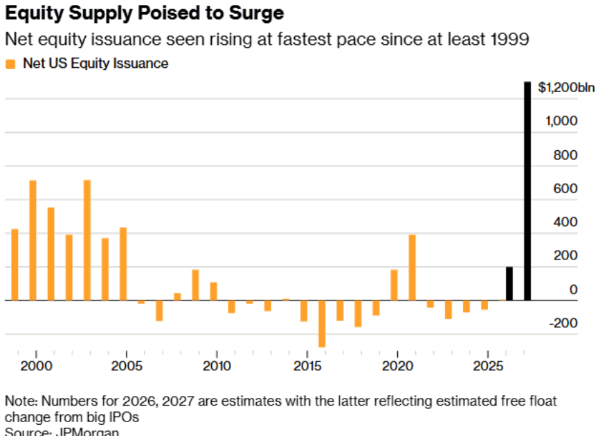
Twenty years of corporate America buying back its own stock built a tailwind nobody named. Since the mid-2000s, net US equity issuance ran negative — roughly $12 trillion in S&P 500 buybacks steadily retired the public float, while automatic passive and 401(k) flows chased an ever-shrinking pool. Fewer shares, same money: prices and multiples climbed on plumbing, not just earnings. That scarcity bid is now set to invert, hard. JPMorgan models net issuance near $1.2 trillion in 2027 — roughly twice the 2000 and 2003 peaks of about $650 billion, the fastest pace since at least 1999, and some $1.5 trillion of net new supply across 2026-27. The driver isn’t operating companies raising cash; the chart note says “free float change from big IPOs” — a decade of private capital converting to public float in one wave: 160-plus filings, over $120 billion in planned raises exceeding the prior two years combined, SpaceX’s roughly $75 billion debut the marquee name. A mega-IPO creates no new wealth; buyers must fund it from the same pool. The standing 401(k) bid must now swallow a flood — unless inflows accelerate to match. The floor turning into the ceiling.
Market Intelligence Brief (MIB) Ver. 18.40
For professional investors only. Not investment advice.
© 2026 RecessionALERT.com
MIB Weekly: Dow Cracked 50,000 and a $2.1T IPO Debuted in the Same Week — Long Semis, Short AI Cash-Burn; Iran Holds the Key to Warsh’s June 17 FOMC
MIB WEEKLY DIGEST
Week of Jun 8–12, 2026
Iran’s 14-point Hormuz draft MoU sent WTI from $91.78 to $84.24 by Friday, potentially deflating the energy surge that drove May CPI to a three-year high (4.2%) and locked out Fed cuts heading into Warsh’s June 17 inaugural FOMC — now with 47% hike odds priced in. SpaceX debuted as the largest IPO in US history ($75B raised, +19.3% at $161 Friday), while Intel’s Google foundry win and JPMorgan’s KLAC upgrade drove the semiconductor equipment complex +20–32% on the week. Oracle’s record $638B cloud backlog failed to prevent a 13.83% weekly loss as its –$23.7B FCF and $40B capital raise plan established a new valuation discipline: AI demand is confirmed, but cash-burn risk is now priced.
TABLE OF CONTENTS
A. WEEK AT A GLANCE
B. WEEK IN MARKETS
C. WEEK’S TOP STORIES (9)
D. WEEK IN THE ECONOMY (5)
E. WEEK IN EARNINGS (1)
F. NEXT WEEK SETUP
G. CHART OF THE WEEK
A. WEEK AT A GLANCE -> TOP
MARKET SNAPSHOT
The S&P 500’s +0.64% WoW gain masks a week of historic volatility: a Dow break below 50,000 on Wednesday (CPI 4.2% + US airstrikes on Iran) fully reversed to a Thursday surge (+1.75%) and Friday calm as a 14-point Hormuz draft MoU circulated. The Iran-US conflict oscillation drove every session’s direction — escalate, ceasefire, collapse, peace signal — and in doing so drove the energy inflation that reset the Fed policy framework: Goldman withdrew its cut forecast, 47% hike odds are now priced, and Warsh inherits a stagflation trap for his June 17 inaugural FOMC. The week’s clearest structural signal came not from the S&P headline but from breadth: Russell 2000 +3.97% and DJTA +3.12% both materially outpaced large-cap indices, confirming the bull market’s foundation is widening beyond AI mega-cap concentration.
THIS WEEK AT A GLANCE
• Biggest weekly swing sessions: Wednesday S&P –1.62% (dual shock: CPI 4.2% three-year high + US-Iran military strikes, Dow cracked 50,000) reversed entirely Thursday +1.75% (Iran peace signal, Nasdaq +3.29%, VIX –12%) — the most complete single-session reversal of a dual macro shock in 2026.
• Biggest weekly winner — KLAC +31.94%: JP Morgan “triple-earner by 2030” upgrade (HBM fab, 3nm/2nm logic, advanced packaging) plus a 10-for-1 stock split effective June 12; the week’s entire top-5 gainer list was semiconductor equipment or foundry names.
• Biggest weekly loser — ORCL –13.83%: Q4 FY2026 earnings revealed –$23.7B FCF and a $40B FY2027 capital raise plan; record $638B RPO and OCI +93% could not offset the financing shock in a 47%-hike-odds rate environment; established a new “prove the GAAP earnings” valuation discipline for AI cloud names.
• Standout commodity — WTI crude –6.65% WoW ($90.24 → $84.24): Iran conflict oscillation drove 4 distinct moves in 5 sessions; Friday’s 14-point Hormuz MoU draft was the week’s primary market-moving catalyst alongside the CPI print.
• Historic IPO — SpaceX (SPCX) +19.3% debut at $161, $2.1T valuation: $75B raised (largest in US history), 2x oversubscribed; S&P 500 profitability-criteria exclusion confirmed — earliest possible inclusion Q3-Q4 2027. The IPO’s $150B institutional demand extracted liquidity from AI mega-cap overweights all week, explaining the top-5 weekly decliners (ORCL, MSFT, PLTR, AAPL, IBM — all Technology sector names).
• Inflation inflection — CPI 4.2% (three-year high, Wed Jun 10) + PPI 6.5% YoY (double consensus, Thu Jun 11): Goldman withdrew its 2026 cut forecast; CME moved to zero cut probability; 47% hike odds locked in. Michigan 5-year inflation expectations fell 50bps to 3.4% Friday (largest single-month drop in years) — the only partial relief signal entering Warsh’s June 17 dot-plot.
KEY THEMES
1. Iran as the Inflation Pivot — The same narrative drove both the worst session and the best session of the week, and it’s the single variable capable of determining the second half of 2026: Hormuz supply disruption drove CPI’s 4.2% headline (gasoline +40.5% YoY), and a confirmed deal with Hormuz reopening would mechanically deflate June and July CPI over 60–90 days — potentially rehabilitating the rate-cut narrative that Goldman abandoned this week. Warsh’s June 17 dot-plot is the first signal of whether the Fed is treating Iran de-escalation as a transitory inflation relief or holding the stagflation posture regardless.
2. AI Capital Cycle at Saturation Scale — The week simultaneously confirmed AI demand at unprecedented scale (SpaceX $150B in orders, Intel Google/NVIDIA foundry wins, Oracle $638B RPO) and revealed that the financing of that demand now exceeds organic cash generation across every major AI infrastructure company (Oracle –$23.7B FCF, SMCI $7B dilution, CoreWeave $6.75B debt). The market’s new valuation discipline is explicit: GAAP-earnings validation is required, guidance raises alone do not hold multiples in a 4.5%+ rate environment. The semiconductor equipment layer — the picks-and-shovels tier with customer-committed demand — is the exception and the week’s clearest structural opportunity.
3. Breadth Widening Beneath Headline Volatility — The S&P’s +0.64% is the week’s most misleading number. Russell 2000 +3.97%, DJTA +3.12%, 10-of-11 sectors green Friday, Consumer Defensives leading three sessions as a stagflation hedge — all point to a bull market foundation that is widening beyond AI mega-cap concentration. Two Market History Signals fired simultaneously this week: DJTA outpaced DJIA by +2.46% WoW (Dow Theory threshold crossed, bullish) and Russell 2000 outpaced S&P 500 by +3.33% WoW (broad participation signal). Both point in the same direction: durable recovery broadening, not narrowing, even as the Iran/Fed narrative creates surface volatility.
B. WEEK IN MARKETS -> TOP
Iran dominated every session: Monday’s missile exchange (WTI to $93) through Wednesday’s US airstrikes and the Dow breaking below 50,000 (VIX 22), then Thursday’s peace-signal reversal (Nasdaq +3.3%, VIX –12%) and Friday’s 14-point draft MoU committing Hormuz reopening within 30 days. That oscillation produced the week’s most anomalous cross-asset read: on Wednesday, 4.2% CPI drove gold –4.49% alongside equities as real yields overrode every geopolitical safe-haven bid — the rate-hike signal dominated the war signal in a single session. The AI crowded-trade unwind ran in parallel: SpaceX’s $75B IPO extracted institutional liquidity from AI overweights all week, driving the semiconductor complex –9% mid-week before JPMorgan and BofA upgrades on Thursday anchored the AI capex thesis and produced an 8% single-session recovery. Breadth is the structural verdict: Russell 2000 (+3.97%) and DJTA (+3.12%) both meaningfully outpaced the S&P 500 (+0.64%) on the week.
FRIDAY CLOSE & WEEK-ON-WEEK CHANGE — Fri, Jun 12, 2026:
MAJOR INDICES
Two Market History Signals fired simultaneously this week. DJTA outpaced DJIA by +2.46 percentage points WoW — above the 2% Dow Theory divergence threshold — but here the split reads bullish: transports priced Iran de-escalation (lower fuel costs) while industrials absorbed Wednesday’s CPI shock before recovering. Russell 2000 extended the participation signal further, outpacing S&P 500 by +3.33% WoW — the clearest breadth confirmation available, with domestic small-caps pricing Iran geopolitical relief the most directly. Both history signals fired in the same direction: durable recovery broadening beyond mega-cap leadership, not narrow tech-only momentum.
| Index | Fri Close | WoW Change | WoW % | Why It Moved (Week) |
|---|---|---|---|---|
| S&P 500 | 7,431.40 | +47.56 | +0.64% | Iran oscillation (Wed dual shock –1.62%, Thu peace reversal +1.75%) netted a modest gain; SpaceX IPO liquidity drain kept AI mega-cap names under distribution pressure through mid-week. |
| Dow Jones | 51,202.29 | +335.51 | +0.66% | Blue-chip composition cushioned the AI selloff; cracked 50,000 Wednesday then recovered above Thursday-Friday; less semiconductor weighting provided partial insulation. |
| DJ Transportation | 22,596.7 | +683.1 | +3.12% | Iran de-escalation cut fuel cost outlook (WTI $90→$84) making logistics and transport the week’s clearest cyclical beneficiary; DJTA posted consecutive 10-session highs Thursday and Friday. |
| Nasdaq 100 | 29,635.95 | +678.35 | +2.34% | Semiconductor equipment surge Thursday-Friday (SOX +8%, KLAC +13%, SNDK +14%) more than offset mid-week AI selloff; SpaceX IPO crowding-out pressure cleared by week-end. |
| Russell 2000 | 2,944.82 | +112.47 | +3.97% | Domestic small-caps immune to Hormuz supply-chain risk outpaced all large-cap indices WoW; +3.33% outperformance vs S&P 500 signals broad market participation confirming the recovery. |
| NYSE Composite | 23,595.79 | +339.29 | +1.46% | Equal-weighted broad market outpaced cap-weighted S&P 500 (+1.46% vs +0.64%), confirming breadth widening beyond mega-cap concentration as Iran fears eased and cyclicals recovered. |
VOLATILITY & TREASURIES
Wednesday’s VIX-to-22 alongside rising 10Y and 2Y was the week’s clearest inflation-fear (not recession-fear) print — in recession scenarios bonds rally and yields fall; here both moved higher with equities lower, confirming policy-tightening fear drove the selloff, not growth collapse. The week’s most telling fixed-income signal came Thursday: when Nasdaq surged 3.3% on the Iran peace deal, the 10-year fell only 8.9 bps — bond markets declined to fully price the geopolitical narrative, holding May’s 4.2% CPI in the other hand. The 2-year at 4.087% Friday still sits 40 bps above the Fed’s policy ceiling, with 47% hike odds intact through all the drama.
| Instrument | Fri Level | WoW Change | Why It Moved (Week) |
|---|---|---|---|
| VIX | 17.69 | –3.88 (–17.99%) | Spiked to 22.22 Wednesday on CPI + Iran dual shock; collapsed on Thursday’s peace signal and Friday’s MoU draft; net WoW lower despite three sessions above 19. |
| 10-Year Treasury Yield | 4.481% | –5.1 bps | Iran de-escalation compressed inflation expectations embedded in yields; soft core CPI (0.2% MoM) provided partial relief; bond market declining to fully price the Iran deal keeps yields elevated. |
| 2-Year Treasury Yield | 4.087% | –6.4 bps | Short end eased slightly as Iran peace narrative outweighed hot PPI/CPI; still 40 bps above Fed’s policy ceiling, pricing near-50% hike probability into year-end. |
| US Dollar Index (DXY) | 99.78 | –0.28 (–0.28%) | Modest safe-haven unwind as Iran risk premium deflated; modestly lower yields weighed; no structural dollar break — net move negligible. |
COMMODITIES
Wednesday’s gold selloff alongside equities during active US-Iran military strikes is the week’s defining anomaly: hot CPI drove real yields sharply higher, which overwhelmed every geopolitical safe-haven bid — the rate-hike signal dominated the war signal in a single session. Thursday—Friday recovered (gold +2.45%, +2.95%) but net WoW gold is –2.71%, confirming real-yield pressure as the structural headwind even against the week’s extreme geopolitical backdrop. Copper’s +3.47% is the corrective signal: industrial metals held and ultimately rallied, sustained by AI infrastructure buildout and electrification demand that proved immune to the week’s macro volatility.
| Asset | Fri Price | WoW Change | WoW % | Why It Moved (Week) |
|---|---|---|---|---|
| Gold | $4,235.42/oz | –$118.13 | –2.71% | Wednesday’s CPI shock drove real yields higher, overriding the war safe-haven bid (–4.49% that session); Thursday—Friday Iran peace narrative restored $200+ of that loss; net WoW negative on rate-pressure dominance. |
| Silver | $68.050/oz | +$0.035 | +0.05% | Massive intraday swings (–4.62% Tuesday, –2.67% Wednesday, +4.16% Thursday, +6.33% Friday) netted essentially flat; dual precious-metal and industrial-demand role produced volatile but balanced outcome. |
| Copper | $6.4783/lb | +$0.2173 | +3.47% | Industrial demand held through the week’s macro turbulence, rising Friday +3.24% on Iran de-escalation; AI infrastructure and electrification buildout providing structural support independent of geopolitical noise. |
| Platinum | $1,718.80/oz | –$60.25 | –3.39% | Precious metals complex weakness from Wednesday’s real-yield spike; auto/industrial demand concerns; partial recovery Thursday—Friday insufficient to offset mid-week losses. |
| Bitcoin | $63,484 | +$2,015 | +3.28% | Pure risk-proxy week — tracked equity direction without independent catalyst; rose Thursday—Friday with the broad risk-on reversal; tracking semis, not leading them. |
ENERGY
Oil’s directional flip mid-week maps precisely to the Iran narrative: Wednesday’s WTI rising alongside collapsing equities was the stagflation signature — supply shock driving both higher oil and market fear simultaneously (a sequence that confirmed the Iran arc is the dominant inflation driver). Thursday—Friday reversed: WTI fell with equities rallying, the classic demand/growth-positive read. The same commodity cannot send both signals in one week without the underlying driver changing — and it did, from war-premium inflation to peace-deal deflation. WTI—Brent spread narrowed from $2.70 to $2.52 as the deal priced out the US-specific supply risk premium; Henry Hub decoupled entirely on a 108 Bcf storage injection.
| Asset | Fri Price | WoW Change | WoW % | Why It Moved (Week) |
|---|---|---|---|---|
| Crude Oil (WTI) | $84.24/bbl | –$6.00 | –6.65% | Iran conflict arc: re-escalation Monday ($91.25) → ceasefire Tuesday ($88.54) → US strikes Wednesday ($91.78) → peace signal Thursday ($86.04) → 14-point MoU Friday ($84.24); each move binary on conflict news, not demand fundamentals. |
| Crude Oil (Brent) | $86.76/bbl | –$6.18 | –6.65% | Same Iran arc; WTI—Brent spread tightened from $2.70 to $2.52 as the deal expectations removed global (not regional) supply premium; Brent led the decline from higher starting-week level. |
| Natural Gas (Henry Hub) | $3.135/MMBtu | –$0.087 | –2.70% | Independent of crude; domestic storage dynamics drove decline (108 Bcf injection Thursday above expectations); seasonal maintenance at LNG export terminals added pressure; no Hormuz connection. |
| Natural Gas (Dutch TTF) | $15.87/MMBtu | –$0.59 | –3.58% | European gas fell on Iran peace hopes; Hormuz reopening expected to restore LNG flows and reduce European supply risk premium; Friday alone –5.87% on MoU draft confirmation. |
S&P 500 SECTORS — WEEKLY ROTATION
Basic Materials’ +3.58% week-lead was a short-covering bounce off its worst 1-month stretch (–4.96%) — mean reversion, not a regime shift, as no fundamental demand catalyst changed for the sector. Technology’s +1.04% WoW is the week’s most misleading number: the top 5 weekly gainers AND top 5 weekly decliners in the movers tables below are all Technology names. Strip the semiconductor equipment complex (+21–32% for KLAC, SNDK, AMAT, LRCX) and the remaining tech names (MSFT, PLTR, AAPL, ORCL) dragged the sector lower — making Technology’s headline this week the broadest intra-sector dispersion of any sector this year, not a signal of directional conviction.
| Sector | 1-Week | 1-Month | 3-Month | 6-Month | YTD | 12-Month |
|---|---|---|---|---|---|---|
| Basic Materials | +3.58% | –4.96% | +4.25% | +18.00% | +14.94% | +41.43% |
| Consumer Defensive | +2.76% | –0.77% | +0.31% | +9.19% | +9.45% | +6.68% |
| Financial | +2.59% | +4.60% | +11.46% | +2.15% | +0.61% | +12.83% |
| Real Estate | +1.82% | +2.46% | +6.94% | +9.85% | +10.69% | +8.36% |
| Industrials | +1.40% | +1.64% | +9.17% | +15.36% | +16.12% | +26.82% |
| Technology | +1.04% | +2.49% | +27.10% | +16.73% | +20.58% | +43.04% |
| Consumer Cyclical | +0.94% | –4.20% | +4.65% | –4.87% | –4.37% | +5.71% |
| Healthcare | +0.87% | +3.11% | +3.22% | +0.80% | –0.59% | +13.33% |
| Utilities | +0.40% | –1.52% | –4.30% | +4.64% | +4.41% | +13.14% |
| Energy | +0.07% | –1.57% | +0.67% | +26.09% | +28.33% | +34.05% |
| Communication Services | –1.52% | –7.20% | +5.78% | +0.64% | +1.31% | +23.68% |
TOP WEEKLY MOVERS:
All five gainers share one catalyst cluster: Intel’s Monday foundry wins (Google 3M+ TPU order, NVIDIA 18A trials) ignited the semiconductor equipment complex, and Thursday’s JPMorgan/BofA upgrades — KLAC triple-earner by 2030, LRCX and AMAT as primary AI capex beneficiaries — locked in institutional conviction. KLAC at +105% half-year and +695% five-year is momentum continuation, not a counter-trend bounce. All five decliners share one mechanism: SpaceX’s $75B IPO forced managers to liquidate the most-overweight AI/tech positions all week — ORCL (FCF burn shock, –$23.7B FCF), MSFT (Xbox restructuring, –19% YTD), PLTR (technical breakdown, –28% YTD), AAPL (WWDC disappointment), IBM (quantum capex skepticism). The leaderboard is a capital displacement event — hardware foundry wins financed by AI software exits — not a fundamental sector split.
TOP 5 WEEKLY GAINERS
| Ticker | Week | YTD | Year | Why It Moved |
|---|---|---|---|---|
| KLAC | +31.94% | +109.48% | +190.90% | JP Morgan upgrade called KLAC a potential “triple-earner” by 2030 driven by HBM fab upgrades, 3nm/2nm logic, and advanced packaging demand; multiple analyst PT increases (Cantor $2,500, UBS $2,180, Barclays $2,250). 10-for-1 stock split also effective this week (shares began trading split-adjusted June 12). |
| SNDK | +26.98% | +734.15% | +4,694.43% | NAND flash shortage driven by AI data-center demand; 251% YoY revenue growth in Q3 2026 and $42B in multi-year supply contracts; BofA raised PT to $2,100; rode the semiconductor equipment upgrade wave with KLAC/AMAT/LRCX. |
| INTC | +25.61% | +237.59% | +499.76% | Monday: Google 3M+ TPU firm manufacturing order + NVIDIA 18A early trials (+11%); Friday: BofA double upgrade (Underperform→Buy) raising 2030 server CPU TAM to $170B, EPS power above $6/share. Two distinct catalysts four days apart. |
| AMAT | +25.22% | +120.73% | +224.14% | Record Q2 2026 results (revenue $7.91B, EPS $2.86, both beat); BofA named primary AI capex beneficiary of the fab upgrade cycle; Mizuho raised PT to $540; $500M Singapore campus expansion announced. |
| LRCX | +20.95% | +114.28% | +300.19% | BofA named primary AI capex beneficiary alongside AMAT; WFE market forecast revised to $140B+ for 2026; advanced packaging revenue growth exceeding 50% in 2026; multiple analyst PT raises (Cantor $425, UBS $375). Intel 18A foundry ramp benefits Lam’s etch and deposition tools directly. |
TOP 5 WEEKLY DECLINERS
| Ticker | Week | YTD | Year | Why It Moved |
|---|---|---|---|---|
| ORCL | –13.83% | –5.53% | –7.87% | Q4 FY2026 earnings (AMC June 10): GAAP EPS miss ($1.45 vs $1.50 est.), –$23.7B FCF, $40B FY2027 capital raise plan. Despite record $638B RPO and OCI +93% growth, the massive debt-funded AI capex overhang triggered a two-day ~15% selloff. Also awarded $395.8M government contract, insufficient to offset the financing shock. |
| MSFT | –6.22% | –19.21% | –18.40% | Xbox restructuring announced (major layoffs, –$500M revenue on $20B cumulative spend, 3% accountability margin); SpaceX IPO liquidity extraction from AI software overweights; AI governance compliance costs (Bowman kill-switch mandate). Down ~8% from Jun 9 all-time high through Friday. |
| PLTR | –5.56% | –27.99% | –5.33% | SpaceX IPO extracted liquidity from AI software plays; failed technical breakout above 200-day MA and descending triangle; UK government contract blocked; no fundamental catalyst — pure crowded-trade rotation toward hardware semis. |
| AAPL | –5.27% | +7.09% | +46.15% | WWDC 2026 (June 8): Siri AI revealed as Google Gemini reskin; stock set 52-week high $317.40 intraday then reversed to –1.87% close; EU DMA blocked Siri AI from European launch (450M users excluded); consecutive daily declines through the week on AI strategy disappointment. |
| IBM | –4.42% | –8.09% | –3.13% | $10B quantum computing bet announced June 8 drove stock lower on capital allocation skepticism; IBM down from its June 2 all-time high $329.23 through week-end; no positive fundamental catalyst offset the sector rotation away from legacy enterprise tech. |
C. WEEK’S TOP STORIES -> TOP
The week’s nine stories form three interlocking threads. The Iran arc (#1) and the CPI/Fed path reset (#2) are causally linked — Hormuz supply disruption drove the energy inflation that eliminated Fed cuts and elevated hike odds to 47%. The AI capital cycle runs through stories #3, #4, #6, and #8, simultaneously validating demand (Intel foundry wins, SpaceX oversubscription) and exposing financing stress (ORCL FCF burn, SMCI dilution). Apple’s WWDC (#5) stands alone as a mega-cap AI strategy failure with index-level weight. All threads converge on one question: whether Iran de-escalation deflates the energy-inflation driver enough to reopen the Fed easing path that Warsh’s June 17 dot-plot must address.
UNCERTAIN
1. Iran War to Draft Peace Deal: Petrochemical Strikes → US Military Response → 14-Point Hormuz MoU — WTI $93.67 to $84.24 in Five Sessions
The core facts:Monday: Israeli-Iranian overnight missile exchange; Mahshahr petrochemical complex struck; ~30 missiles fired at Israel; WTI surged to $93.67; OPEC+ approved +188K bpd July increase (“symbolic” given Hormuz); Trump claimed imminent ceasefire. Tuesday: Iran-Israel halted attacks; nuclear talks advancing; WTI –4.04% to $87.61; but Hormuz blockade persisted and an Iranian Apache helicopter downing complicated the truce. Wednesday: Ceasefire collapsed entirely; US struck Iranian air defense sites; Iran retaliated against US regional bases; Trump stated “we’re going to be attacking them very hard” and signaled civilian-infrastructure strikes; WTI +4.06% to $91.78; Dow broke below 50,000. Thursday: Trump cancelled strikes via Truth Social; announced imminent peace signing; Dow +1.86%, Nasdaq +3.29%, WTI –4.43% to $86.04, VIX –12.47%. Friday: Iran’s Mehr News Agency confirmed a 14-point draft MoU — Hormuz reopening within 30 days, oil sanctions lifted, ~$25B frozen assets released — but Trump and Iranian officials published incompatible accounts of deal terms. WTI fell to $84.24. The Strait of Hormuz remained under dual US-Iran blockade removing 11M+ bbl/day throughout the entire week.
Why it matters:The Hormuz supply disruption was the primary driver of May CPI’s 4.2% headline (gasoline +40.5% YoY, energy +23.5% YoY). Every session’s market direction — including the anomalous Wednesday gold selloff alongside equities — traced back to whether Iran deal signals were advancing or collapsing. A confirmed deal with Hormuz reopening would mechanically deflate June and July CPI over the following 60–90 days, potentially rehabilitating the rate-cut narrative that Goldman abandoned June 7. The execution risk remains extreme: two sides published incompatible deal terms, a fresh drone attack complicated the timeline, and the Strait remained physically blocked as of Friday close. UNCERTAIN classification reflects that the week ended with a peace signal but not a peace fact. (WTI –6.65% WoW — see Energy table in Section B above.)
What to watch:Formal signing ceremony with both sides present; WTI sustained below $85/bbl as supply-premium confirmation; Hormuz AIS vessel-tracking for corridor reopening within the 30-day window; whether the deal holds through Warsh’s June 17 FOMC.
BEARISH
2. May CPI 4.2% Three-Year High + PPI 6.5% Double Consensus — Goldman Withdraws Cut Forecast; 47% Hike Odds; Warsh Inherits the Stagflation Trap
The core facts:Wednesday June 10: BLS reported May CPI at 4.2% YoY (three-year high, third consecutive monthly acceleration), with energy accounting for >60% of the monthly gain (gasoline +40.5% YoY). Core CPI 0.2% MoM (below 0.3% consensus) — the only narrow relief. Goldman Sachs formally withdrew its 2026 rate-cut forecast and raised hike probability to 20%. CME FedWatch moved to zero probability of any 2026 cut. Thursday June 11: BLS reported May PPI +1.1% MoM (double the 0.7% consensus), 12-month rate 6.5% (highest since November 2022), driven by wholesale energy +10.7% MoM. Initial jobless claims 229K (highest since February, above 219K consensus). The dual PPI + claims data created the week’s policy trap: inflation too hot to cut, labor too soft to hike confidently. By Friday: Polymarket and Kalshi hike odds at 47%; 2-year Treasury at 4.087% (40 bps above the Fed’s policy ceiling); Michigan 5-year inflation expectations fell 50 bps to 3.4% — the only partial relief signal, giving Warsh analytical cover for a hawkish pause.
Why it matters:The CPI print eliminated any residual rate-cut possibility for 2026 and elevated hike probability to near coin-flip odds — the most significant monetary policy shift of the year. With FOMC blackout in force from Saturday June 7 through June 17, Warsh has had zero opportunity to communicate to markets; the June 17 dot-plot arrives as the first mandatory reset point for every duration position heading into H2 2026. The soft core CPI (0.2% MoM) and Friday’s Michigan 5-year expectations drop to 3.4% argue domestic inflation is more contained than the headline suggests — if Iran de-escalation removes the Hormuz energy driver, June CPI could drop sharply. But if the deal fails, the pipeline (PPI 6.5% YoY) flows through for at least two more monthly prints. (2Y at 4.087%, 10Y at 4.481% — see Vol & Treasuries table; Polymarket hike odds 53%→47% WoW — see Polymarket table in Section D.)
What to watch:June 17 FOMC dot-plot — any median above 3.75% formally marks the end of the easing cycle; Warsh’s inaugural press conference for the first explicit rate-path signal; June CPI (July 14) for whether Iran oil deflation flows through.
BULLISH
3. Intel Foundry Transformation Validated: Google 3M+ TPU Order + NVIDIA 18A Trials Monday; JPMorgan + BofA Upgrades Thursday; SOX +8% in Single Session
The core facts:Monday June 8: Google placed a firm order for >3 million TPUs to be manufactured by Intel’s foundry in 2028; NVIDIA is running early trials of Intel’s 18A process node for its next-generation Feynman GPU architecture (no firm contract yet). INTC +11.11%; KLAC +9.21%, AMAT +8.61%, MU +9.87% swept higher. Thursday June 11: JP Morgan upgraded KLA Corporation, citing potential to triple earnings by 2030 from HBM fab upgrades, 3nm/2nm logic, and advanced packaging demand; Bank of America simultaneously named Lam Research and Applied Materials as primary AI capex beneficiaries; the Philadelphia Semiconductor Index (SOX) surged ~8% — its single-session strongest gain since early 2025; Lam’s WFE market forecast raised above $140B for 2026. Friday June 12: BofA double-upgraded Intel directly from Underperform to Buy, raising 2030 server CPU TAM to $170B and EPS power above $6/share; INTC +6.48% Friday. Weekly totals: INTC +25.61%, KLAC +31.94%, AMAT +25.22%, LRCX +20.95%, SNDK +26.98%.
Why it matters:For three years, Intel Foundry Services has been the central investment thesis driving INTC’s ~250% YTD rally — manufacturing ambitions require commercial validation. Google placing a 3M+ TPU order and NVIDIA running 18A trials provides exactly that: the two most consequential AI hardware customers have committed real capital. The JPMorgan and BofA analyst upgrades Thursday are structurally significant: they establish semiconductor equipment as a multi-year secular growth story tied to AI capex, with the $140B+ global WFE market providing KLAC, LRCX, and AMAT returns analogous to NVDA’s prior-cycle trajectory. The week showed the underlying AI capex demand is intact — what the mid-week selloff revealed was a crowded-position flush, not a fundamental deterioration. (See top weekly gainers table in Section B above — all five gainers are semiconductor equipment/foundry names.)
What to watch:Any firm NVIDIA 18A manufacturing contract announcement (converting “early trials” to “signed order”); Intel Q2 FY2026 earnings (late July); NVDA Q2 FY2027 earnings (August) as the next major AI demand anchor.
BULLISH
4. SpaceX (SPCX) Prices $75B — Largest IPO in US History; Debuts +19.3% at $161 / $2.1T Valuation; S&P 500 Exclusion Removes Near-Term Passive Catalyst
The core facts:Tuesday: SpaceX confirmed $150B+ in institutional orders (2x oversubscribed) ahead of June 11 pricing. Thursday June 11: SpaceX priced at $135/share, raising $75 billion — the largest single equity raise in US capital markets history. BlackRock placed a single ~$5B order. Friday June 12: SPCX opened at $150, closed at $161.11 (+19.3%) on 360M+ shares; at $2.1T market cap, briefly made Elon Musk the world’s first trillionaire on combined Tesla+SPCX stake. S&P Dow Jones Indices confirmed no change to GAAP profitability criteria; earliest possible S&P 500 inclusion is Q3-Q4 2027 — removing the $200-400B passive-buying catalyst many investors had been pricing in. Nasdaq-100 has rewritten eligibility rules and expects to include SPCX on a faster timeline. The IPO closed alongside Anthropic (S-1 June 1), OpenAI (S-1 June 8), completing the AI/frontier-tech public-markets pipeline in 11 days.
Why it matters:$150B in demand against $75B raised — 2x oversubscribed amid CPI at 4.2%, VIX spiking to 22, and a hawkish FOMC week — confirms institutional risk appetite is intact for transformational infrastructure assets even under macro stress. The $75B extraction from existing institutional positions explains all five names in the weekly decliners table (ORCL, MSFT, PLTR, AAPL, IBM): portfolio managers liquidated AI overweights to fund SPCX allocations. The S&P 500 exclusion is a structural negative for the valuation thesis: passive index inflows anticipated at $200-400B do not arrive on any near-term timeline. The Anthropic/OpenAI pipeline means a sustained new-supply overhang on AI institutional allocations extends well into 2026-2027.
What to watch:Nasdaq-100 inclusion decision (weeks, not months); SPCX trading above $135 IPO price as demand-absorption confirmation; S&P 500 profitability milestones in SpaceX’s first four public quarters; Anthropic and OpenAI IPO timelines as the next supply-overhang events.
BEARISH
5. Apple WWDC 2026: Siri AI as Google Gemini Reskin Reversed a 52-Week Intraday High; EU DMA Then Blocked the Launch for 450M European Users; AAPL –5.27%
The core facts:Monday June 8 (WWDC): Apple unveiled iOS 27 headlined by a revamped Siri AI powered in part by Google Gemini — an explicit concession that Apple cannot build frontier AI at required pace internally. Shares rallied 3%+ to a 52-week high of $317.40 intraday, then reversed during the keynote to close –1.87% at $301.60 — a ~5% intraday swing peak to close. Barclays reiterated Underweight ($253 PT); UBS maintained Neutral. Tuesday June 9: Apple confirmed Siri AI will not be available in the EU at iOS 27 launch, citing the Digital Markets Act — approximately 450 million European users excluded. AAPL fell an additional –3.70% Tuesday. By Friday: AAPL at $291.08, –5.27% on the week from the prior Friday’s close.
Why it matters:The 52-week-high-to-reversal intraday pattern is the clearest possible market verdict: the sell-on-news reaction to WWDC was not forced by external macro factors but by the announcement’s content. The iPhone supercycle thesis — the primary bull case supporting Apple’s elevated multiple — requires Apple Intelligence to compel a global upgrade cycle. The EU ban structurally removes 25-30% of the premium smartphone market from that trigger. The two-day cumulative decline from the intraday high ($317.40) to Tuesday close ($290.38) represents ~$220B in market cap loss from the world’s largest company, with direct S&P 500 index-weight consequences. The longer-term risk: if Siri AI is perceived as a Google Gemini reskin rather than a proprietary intelligence layer, Apple’s premium moat in the market narrows structurally. (See weekly decliners table in Section B above.)
What to watch:Whether Apple pursues a DMA legal challenge or privacy-preserving interoperability framework — both measured in months. Analyst rating changes in the next 7-10 days. iPhone 17 pre-order data September as the first hard upgrade-cycle signal.
BEARISH
6. AI Capex Exceeds Cash Generation: Oracle –$23.7B FCF + $40B Capital Raise; SMCI $7B Dilutive Offering — Both on $39B+ in Confirmed AI Demand
The core facts:Wednesday June 10 AMC: Oracle (ORCL) reported Q4 FY2026 — record RPO $638B (+53% YoY), OCI +93% growth, non-GAAP EPS $2.11 (beat) — but GAAP EPS missed ($1.45 vs $1.50 est.), FY2026 free cash flow was negative $23.7 billion, and Oracle announced a ~$40 billion FY2027 capital raise plan including a $20B ATM equity issuance. ORCL fell –7.12% AH Wednesday, then –8.53% Thursday — a two-day cumulative ~15% decline on a quarter that reported record cloud metrics. Wednesday evening: Super Micro Computer (SMCI) announced $7 billion equity and equity-linked financing to fund component procurement for $39B in AI server backlog from 20+ customers. SMCI fell ~9.5% AH, then –17% Thursday — erasing ~$12B in market cap on demand confirmation. Simultaneously Thursday: CoreWeave priced $1.25B + €2B in senior notes and announced $3.5B additional offering — $6.75B in AI debt financing in a single session.
Why it matters:Oracle’s –$23.7B FCF against a $638B RPO is the sharpest illustration of the AI infrastructure financing paradox available: the demand is real and enormous, but the capital required to fulfill it exceeds organic cash generation by a massive margin. When even a $500B enterprise software company cannot self-fund its AI buildout from operations, equity and debt markets become the capital source — creating a sustained dilution overhang across the AI cloud infrastructure complex. SMCI’s separate $7B raise arrived the same night, compounding the “AI capex is dilutive” narrative into a sector-wide signal that drove the mid-week selloff (QCOM –6.92%, AVGO –5.12%, MRVL –5.35%). The broader implication: the AI infrastructure cycle has entered a phase where even confirmed demand cannot prevent significant stock punishment if execution requires equity dilution or FCF deterioration.
What to watch:Oracle Q1 FY2027 earnings (September) — first FCF trajectory signal; CoreWeave high-yield credit spreads as the leveraged AI infrastructure financing marker; SMCI execution against the $39B backlog in the next quarterly update.
UNCERTAIN
7. White House Declares US-China Trade Deal “Done” — 30% Tariff Baseline Locked, Rare Earth Shipments Resume; Beijing Calls It a “First Meeting Framework”
The core facts:Thursday June 11: The White House announced a finalized US-China trade framework: the US maintains a 30% aggregate tariff on Chinese goods (20% “fentanyl” + 10% “reciprocal”); China maintains a 10% baseline on US goods; US resumes full acceptance of Chinese students; China agrees to resume rare earth and rare earth compound shipments — critical for semiconductor packaging, defense electronics, EV motors, and advanced manufacturing. Pakistan and Qatar served as primary mediators. Beijing characterized the announcement differently — describing it as a “first meeting framework,” not a comprehensive final agreement. Wednesday context: Trump separately announced the US is “not looking to renew” the USMCA before the July 1 review milestone, threatening $1.8T in annual North American trade with Canada and Mexico with the most uncertainty since the trade architecture was established.
Why it matters:Rare earth resumption is the most immediately market-relevant provision: China’s rare earth retaliatory lever — a material cost and supply risk for semiconductor manufacturers and defense contractors — is ostensibly lifted. However, the 30% tariff rate on Chinese goods remains unchanged — this is a tariff freeze, not a rollback. The interpretive divergence between “done” (White House) and “first meeting framework” (Beijing) is the key risk: if China views this as a starting point for further negotiation, the supply-chain confidence markets priced Thursday may prove premature. The USMCA non-renewal threat, arriving the same week as the China framework, means two major trade architectures simultaneously face uncertainty — North American supply chains face regulatory ambiguity that capitals allocation decisions cannot ignore.
What to watch:Whether rare earth shipments actually resume in volume within 30 days; any Chinese statement upgrading from “framework” to “final agreement”; USD/CNY and CNH offshore yuan as real-time deal confidence indicators; July 1 USMCA review deadline as the next North American trade trigger.
BULLISH
8. Marvell Technology Joins S&P 500 on June 22 — MRVL +9% Monday; Forced Passive Buying at $247B Cap from ~$50 in 2024
The core facts:Monday June 8: S&P Dow Jones Indices announced Marvell Technology (MRVL) will join the S&P 500 effective before open on June 22, 2026, replacing Pool Corporation (POOL) and Campbell’s Company (CPB). MRVL surged ~9-10% Monday, trading around $288 at a ~$247B market cap — making it one of the largest additions to the index in 2026. MRVL was up approximately 210% year-to-date at the time of announcement, driven entirely by AI networking chip demand. The stock had traded below $50 entering 2024 — a $200B market cap creation in under two years entirely from AI infrastructure demand.
Why it matters:S&P 500 inclusion is a mechanical passive-demand event: every index fund, ETF, and index-benchmarked institutional mandate must build a MRVL position before June 22. At $247B, the required passive purchases represent a significant known demand event in a week that is simultaneously absorbing the SpaceX IPO. The timing signal is analytically rich: MRVL enters the S&P 500 in the same week it fell –7.61% Tuesday (as SpaceX IPO drained AI liquidity) — index-inclusion provides a structural demand floor that passive managers cannot ignore regardless of weekly volatility. More broadly, MRVL’s rise from <$50 to ~$290 validates that the AI semiconductor boom has created new index-eligible companies at the $200B+ scale that did not exist 24 months ago, reshaping S&P composition at an accelerating pace.
What to watch:MRVL price action through the June 22 addition date; other AI semiconductor names (KLAC post-split, SNDK) as potential future S&P rebalancing candidates as their market caps cross eligibility thresholds.
BULLISH
9. GSK Acquires Nuvalent for $10.6B at 40% Premium — NUVL +39%; Two FDA-Tracked NSCLC Assets in 2026 Approval Window Validate Oncology Buyout Valuations
The core facts:Tuesday June 9: GSK plc announced a $10.6 billion all-cash acquisition of Nuvalent (NUVL) at $124/share — a 40% premium to Monday’s close. The acquisition includes two late-stage NSCLC assets: zidesamtinib (ROS1 inhibitor) and neladalkib (ALK inhibitor), both under FDA review with potential 2026 approvals; plus Ris-Rez (B7-H3 antibody-drug conjugate). NUVL surged ~39%. GSK CEO Luke Miels’ largest acquisition in over a decade; expected to be accretive to core EPS in 2029 inclusive of synergies; deal expected to close Q3 2026.
Why it matters:A 40% all-cash premium for pre-commercial oncology assets sends a clear valuation signal across the biopharma M&A landscape: major pharma is willing to pay buyout-level premiums for best-in-class NSCLC assets while still in the regulatory pipeline, before commercial revenue is established. Three portfolio read-throughs: (1) the ROS1/ALK inhibitor class commands premiums before first approval, validating mid-cap oncology pipeline valuations broadly; (2) oncology M&A competition is active — multiple large-cap names are simultaneously deploying cash for targeted pipeline acquisitions; (3) US oncology names with similar FDA-tracked NSCLC or solid-tumor platforms (Blueprint Medicines, peers) become implicit acquisition targets at comparable multiples. For the broader healthcare sector: M&A is providing a floor for healthcare valuations at a moment when the sector’s YTD return is –0.59% — one of the weakest in the S&P.
What to watch:FDA review timelines for zidesamtinib and neladalkib in 2026; peer oncology M&A activity in the ALK/ROS1 inhibitor space; Blueprint Medicines (BPMC) and similar mid-cap oncology names for comparable premium re-rating.
D. WEEK IN THE ECONOMY -> TOP
The week delivered a textbook stagflation pulse: CPI 4.2% (three-year high) and PPI 6.5% YoY (2× consensus) arrived in the same 48 hours as jobless claims at a four-month high (229K) and NFIB price plans at 34% (4-year high). Core CPI’s 0.2% MoM confirms inflation is Hormuz-energy-driven — but NFIB’s small-business price intentions signal that energy costs are bleeding forward into domestic pricing pipelines for months ahead. Markets resolved the trap into an awkward equilibrium: Polymarket hike odds fell 6pp WoW (Iran de-escalation may deflate the energy-inflation trigger) while cut odds collapsed 25pp (the disinflation narrative is dead), leaving “extended hold” as the modal outcome. Michigan 5-year inflation expectations’ 50-basis-point drop to 3.4% — the largest single-month decline in years — confirms long-run anchoring remains intact, giving Warsh analytical cover to hold without being forced to hike. Wednesday’s FOMC dot-plot is the only instrument capable of resolving the ambiguity: whether Warsh signals a hike path or accepts Iran de-escalation as the transitory relief that keeps rates on hold through 2026.
POLYMARKET ODDS — WEEK-ON-WEEK SHIFT:
| Market | Last Friday | This Friday | Δ |
|---|---|---|---|
| US Recession by end-2026 | 19% | ~19% | 0 pp |
| Fed rate hike in 2026 | 53% | 47% | –6 pp |
| Fed rate cuts ≥1 in 2026 | 28% | ~3% | –25 pp |
BEARISH
May CPI 4.2% Three-Year High + May PPI 6.5% YoY Double Consensus — Energy Dominates Both; Core Data Offers Narrow Relief (BLS, Jun 10–11, 2026)
What they’re saying:CPI: Headline +4.2% YoY (0.5% MoM), highest since April 2023; energy +3.9% MoM (gasoline +40.5% YoY, energy +23.5% YoY). Core CPI: 0.2% MoM (below 0.3% consensus), 2.9% YoY — shelter slowed to 0.3% MoM; new vehicles, furniture, and pharmaceuticals posted first monthly price declines in 14 months. PPI: +1.1% MoM (double the 0.7% consensus, second consecutive month), 6.5% YoY (highest since November 2022); energy +10.7% MoM, gasoline +23.4% wholesale. Core PPI: 0.4% MoM, 4.9% YoY — below the 5.4% consensus.
The context:Both headline prints are Hormuz-driven: if the Iran draft MoU delivers Strait reopening within 30 days, the June–July CPI and PPI headlines mechanically deflate as the gasoline surge reverses. The soft core (CPI 0.2% MoM, PPI core 4.9% YoY below consensus) is the analytically important reading — domestic inflation is more contained than headlines suggest. But NFIB price plans at 34% (4-year high) argue energy costs are bleeding into small-business pricing intentions for months ahead, meaning core may not stay soft. Goldman Sachs withdrew its 2026 cut forecast during this data sequence; CME FedWatch moved to zero cut probability. (10Y at 4.481% Friday — see Vol & Treasuries table in Section B.)
What to watch:June CPI (July 14) as the first read showing whether Hormuz oil deflation flows through into the headline; core PCE (June 26) for the Fed’s preferred measure; June PPI (mid-July).
BEARISH
Goldman Sachs Withdraws All 2026 Rate-Cut Forecasts; Raises Hike Probability 20%; 72 of 102 Economists Now Project Rates Held Flat for All of 2026 (Multiple, Jun 7–12, 2026)
What they’re saying:Goldman Sachs formally withdrew its 2026 rate-cut forecast on June 7, raising near-term hike probability to 20%. A Reuters survey of 102 economists (conducted June 4–9) found 72 now project rates held flat at 3.50–3.75% for all of 2026 — the most unified “hold” consensus of the year. Mohamed El-Erian (Allianz) stated “neither hikes nor cuts” is appropriate given the Hormuz-energy-driven inflation dynamic. CME FedWatch moved to zero cut probability. Polymarket hike odds: 47% at Friday close, down from 53% last Friday (Hormuz de-escalation reducing near-term urgency) but still above the 50% threshold that signals near-coin-flip for the year.
The context:Goldman’s reversal closes the institutional debate: the disinflation narrative that had kept cuts on the table through mid-2026 is formally withdrawn by the bank that was most consistent in forecasting them. The 102-economist consensus at 72/102 for “hold flat all year” means the baseline rate path is now effectively locked — only a dramatic change in either inflation data (Hormuz deal delivers major oil price decline) or growth data (claims surge past 260K) would reopen the debate. For equity managers, the cut narrative is dead and cannot be resurrected by the June 17 FOMC meeting under any realistic outcome — rate-sensitive sector positioning (REITs, utilities, long-duration growth) must be sized for a rates-on-hold environment through at least year-end.
What to watch:June 17 FOMC dot-plot — median rate projection above 3.75% formally resets equity duration positioning; Warsh’s press conference language on Iran as “transitory” vs “structural” inflation as the signal for whether the hike probability rises or holds at 47%.
UNCERTAIN
Initial Jobless Claims 229K — Four-Month High + NFIB Price Plans 34% — Four-Year High: The Dual-Mandate Conflict in Two Data Points (DOL + NFIB, Jun 9–11, 2026)
What they’re saying:Initial claims for week ending June 6: 229K, highest since February, above 219K consensus; continuing claims 1,795K (above 1,780K est.); 4-week moving average 219K (rising trend confirmed). NFIB May: Optimism Index 95.3 (below 98.0 long-run average); net 34% of owners planning price increases (up 7pp from April, highest since July 2022); net 36% raised selling prices in May (highest since March 2023); Uncertainty Index 91 (vs 68 historical average); job openings 29%, down 5pp from April — the lowest since May 2020.
The context:Claims rising + NFIB price plans surging in the same week is the purest available expression of the dual-mandate conflict. For the Fed, this data argues simultaneously against cutting (small businesses raising prices at 4-year pace) and against hiking (labor market showing first consistent softening signals of 2026). NFIB’s job openings at a 6-year low is separately important: small businesses are hiring less even as they raise prices — the classic stagflationary configuration at the most granular labor-market level, one that historically precedes aggregate slowdowns by 1–2 months. UNCERTAIN classification reflects genuine analytical ambiguity: the data is bearish for growth and for Fed easing, but not unambiguously bearish for equities if the Iran deal can remove the energy inflation trigger.
What to watch:Next Thursday claims (June 18, day after FOMC) — sustained above 230K shifts narrative from marginal softening to labor deterioration; June NFIB (~July 8) for whether price intentions hold as gas prices decline post-Iran-deal.
BULLISH
Existing Home Sales 4.17M — Highest Since December Despite 4.55% Yields (NAR, Jun 9); Michigan Sentiment Beats 48.9 With 5-Year Expectations Plunging 50bps to 3.4% (UMich, Jun 12); GDPNow Q2 3.3%
What they’re saying:Existing home sales rose 3.2% MoM in May to 4.17M (SAAR), beating the 4.07M consensus — strongest since December 2025. Midwest led (+6.4%), median price $429,300, inventory 4.5 months. Michigan Consumer Sentiment preliminary June: 48.9, beating 46.0 consensus and up from 44.8 May — first increase in four months; 1-year inflation expectations eased 4.8→4.6%; 5-year expectations fell from 3.9% to 3.4% — the largest single-month drop in years, driven primarily by easing gasoline prices from Iran de-escalation. GDPNow Q2 estimate: 3.3% as of June 9, up from 3.0% (partial recovery from May’s 4.3% peak, still above trend).
The context:Three data points collectively argue the US economy is absorbing the stagflation shock without a demand collapse. Housing beating at 4.55%+ yields signals demand durability that rate levels alone cannot predict — buyers have adjusted to the higher-rate environment. The Michigan 5-year expectations drop to 3.4% is the most analytically Fed-important reading this week: long-run anchoring at 3.4% confirms the Fed’s 2% target is still credible in consumer expectations despite the 4.2% CPI headline, directly providing Warsh the analytical cover he needs to hold rates rather than hike at his June 17 inaugural meeting. GDPNow at 3.3% signals above-trend growth — which simultaneously argues the economy doesn’t need rate cuts, and can tolerate a hawkish hold posture.
What to watch:GDPNow June 16 update (FOMC opening day) as the real-time growth read entering the decision; July Michigan reading as first post-FOMC consumer confidence signal; Q2 GDP first estimate (late July).
BEARISH
GoHealth Chapter 11 ($917M in Liabilities) + Freedom Forever Chapter 11 ($500M+ Debt) — Medicare Advantage + Residential Solar Stress Signal Credit Stress Widening Beyond Rate-Sensitive Real Estate
What they’re saying:GoHealth (GOCO), one of the largest US Medicare Advantage enrollment platforms, filed Chapter 11 June 7 with assets $500M–$1B and liabilities $1B–$10B; prepackaged filing with 100% lender support; expected to emerge before the 2026 Annual Enrollment Period (October 15). Freedom Forever, the second-largest US residential solar installer (6.1% market share), filed Chapter 11 with $500M+ in debt; creditors include Mosaic Funding IX ($100M+), JA Solar, Trina Solar, and Jinko Solar.
The context:Two Chapter 11 filings from adjacent but distinct sectors (healthcare distribution + residential solar) share a common underlying driver: rate-sensitive financing structures that cannot service debt in the current 4.5%+ rate environment, combined with regulatory or demand shocks that removed top-line visibility. GoHealth’s collapse reflects broader Medicare Advantage structural stress — rising MA medical costs and CMS broker compensation rule changes — that is simultaneously compressing carrier margins at Humana, UnitedHealth, and CVS/Aetna. The combined message: credit stress is widening beyond purely rate-sensitive real estate into operating businesses across sectors that relied on 2020–2023 funding conditions. The six-consecutive-year rise in large corporate bankruptcies appears to be accelerating into sectors where federal program expansion created leverage that normalized rate environments cannot sustain.
What to watch:GoHealth emergence timeline before October AEP; Humana (HUM) and UnitedHealth (UNH) Q2 earnings (July) for updated MA medical cost guidance; SunRun (RUN) as the primary residential solar read-through; Q2 corporate bankruptcy rate for trend confirmation.
E. WEEK IN EARNINGS -> TOP
TOP EARNINGS OF THE WEEK
UNCERTAIN
1. Oracle (ORCL): –13.83% week | Record Backlog Meets $23.7B FCF Deficit — AI Cloud Demand Confirmed, Execution Risk Elevated
The Numbers:Q4 FY2026 (AMC Wednesday June 10): Revenue $19.2B (+21% YoY), beat $19.1B est. Non-GAAP EPS $2.11 (+24% YoY), beat $1.96 est. by 7.7%. GAAP EPS $1.45, missed $1.50 est. Cloud revenue $9.9B (+47% YoY); Oracle Cloud Infrastructure (OCI): +93% YoY; SaaS: +10% YoY. Remaining Performance Obligations (RPO): $638B (+53% YoY), including $75B prepaid or customer-supplied AI hardware. FY2026 free cash flow: negative $23.7B. FY2027 guidance: revenue $90B reaffirmed, non-GAAP EPS $8.05 raised; Q1 FY2027 cloud guidance +57–64%. Stock reaction: –7.12% AH Wednesday, –8.53% Thursday regular session, –13.83% week total.
The Problem/Win:The win is unambiguous: OCI at +93% growth, $638B RPO up 53%, and $75B in prepaid AI hardware represent genuine hyperscale competitive traction. Oracle has successfully positioned itself as the AI infrastructure platform for enterprise, competing directly with AWS and Azure at scale. The problem is equally clear: generating –$23.7B in free cash flow while announcing a $40B FY2027 capital raise plan sends the market a financing-risk signal that overwhelms even record cloud metrics. The GAAP EPS miss ($1.45 vs $1.50 est.) reflects the accelerating gap between adjusted profitability and GAAP reality as stock-based compensation and capex expand. A –15% two-day decline on a quarter with a guidance raise is the market’s verdict: “show me GAAP earnings,” not backlog.
The Ripple:OCI’s +93% growth is a competitive read-through to AWS, Azure, and Google Cloud — institutional AI workloads are distributing across multiple hyperscaler platforms. For AWS (AMZN) and Azure (MSFT), Oracle’s growth is market expansion, not market loss. However, ORCL’s selloff on a guidance raise sent a broader signal that was simultaneously absorbed by SMCI, QCOM, AVGO, and MRVL in the same 24-48 hours: the AI capex cycle has entered a “prove the GAAP earnings” phase where guidance raises without GAAP-beat confirmation cannot hold multiples. The –$23.7B FCF profile also adds to the CoreWeave debt raise and SMCI dilution as converging data points that AI infrastructure capital is now a leveraged, multi-player financing cycle, not a self-funding one.
What It Means:Oracle’s AI cloud demand is real — $638B in RPO is not speculative. But the –13.83% weekly loss on record metrics and raised guidance establishes a new valuation discipline for AI cloud names: GAAP-earnings validation is now required, not optional, in a 4.5%+ rate environment. This is a multiple-compression signal that extends to any AI infrastructure name carrying large non-GAAP/GAAP gaps alongside elevated capex.
What to watch:Oracle Q1 FY2027 earnings (September) — first FCF trajectory read; OCI revenue growth deceleration below 80% YoY as the key inflection watch; $40B capital raise execution and its GAAP dilution impact on FY2027 earnings per share.
WEEK AHEAD PREVIEW:
Q1 2026 earnings season is effectively complete (~99% of S&P 500 reported). The coming week’s focus shifts entirely to the June 16–17 FOMC — Warsh’s inaugural decision — with just one mega-cap earnings reporter in the window.
Progressive Corp (PGR) — BMO, Wednesday June 17 — Key focus: Q2 2026 combined ratio trajectory (Q1 came in at 86.0, below the company’s 88.5% long-run average, signaling strong underwriting discipline); premium rate adequacy vs. elevated claims inflation from energy and auto repair costs; policy-in-force growth sustainability (Q1 personal lines PIF +9% YoY). Reports on the same day as the FOMC rate decision — any guidance language on macro uncertainty or pricing power will be read against the day’s monetary policy backdrop. EPS est: $3.75 (non-GAAP), Revenue est: $21.69B.
No other mega-cap earnings are scheduled for the week of June 16–19. Q2 2026 earnings season begins in mid-to-late July 2026.
F. NEXT WEEK SETUP -> TOP
UPCOMING RELEASES:
| Date | Event | Why It Matters |
|---|---|---|
| Mon, Jun 15 | Capacity Utilization (exp. 76.2%, prior 76.1%) | Slack in industrial capacity matters for the inflation debate — utilization near 76% signals room before supply-side pressure emerges; any upside surprise would reinforce the stagflation narrative entering FOMC deliberations. |
| Mon, Jun 15 | Industrial Production MoM (exp. +0.2%, prior +0.7%) | A deceleration from April’s +0.7% would signal the manufacturing sector is absorbing the Iran energy shock; weakness here strengthens the hold case at the FOMC ahead of Wednesday’s decision. |
| Mon, Jun 15 | NAHB Housing Market Index (prior 37) | Builder sentiment at multi-year lows reflects the rate shock; any improvement or further deterioration frames the rate-sensitive sector’s health heading into Warsh’s first rate decision. |
| Tue, Jun 16 | Building Permits Prel (exp. 1.41M, prior 1.423M) | Forward-looking housing demand indicator; a decline from 1.423M would confirm the rate-sensitive sector continues to contract under elevated yields, adding to Warsh’s “growth softening” evidence the day before the FOMC decision. |
| Tue, Jun 16 | Housing Starts (exp. 1.44M, prior 1.465M) | Actual construction activity; a miss below 1.44M alongside the NAHB sub-40 reading would form a consistent housing contraction narrative arriving directly on FOMC Day 1. |
| Tue, Jun 16 | Import/Export Prices MoM (Import prior +1.9%, Export prior +3.3%) | Released on FOMC Day 1; import prices are the pipeline gauge for domestically imported inflation — any sustained elevation above the prior month’s already-hot prints arrives directly into FOMC deliberations. |
| Wed, Jun 17 | FOMC Rate Decision (exp. hold 3.50–3.75%) + SEP Dot Plot | Chair Warsh’s inaugural decision and first dot-plot: any median rate projection above 3.75% formally ends the easing cycle thesis and requires portfolio managers to reset duration exposure across fixed income and equity; the SEP’s longer-run neutral rate estimate is the secondary signal. |
| Wed, Jun 17 | Warsh Inaugural Fed Press Conference 2:30 PM | The market’s first live read of Warsh’s policy communication style and tolerance for above-target inflation; any acknowledgment that Iran de-escalation alters the H2 inflation trajectory would be dovish-at-the-margin and signal the Fed is not mechanically data-locked into hiking. |
| Wed, Jun 17 | Retail Sales MoM (exp. +0.5%, prior +0.5%) | The most important coincident growth read of the week; released before the FOMC statement — a miss would arrive alongside the rate hold as confirmation that rate-sensitive consumer spending is softening, stacking the stagflation signal on the day of the decision. |
WHAT TO WATCH NEXT WEEK:
1. Will Warsh’s dot-plot formalize a rate-hike path? If any committee member raises their median rate projection above 3.75%, it formally ends the easing-cycle thesis and triggers mandatory duration repositioning across institutional fixed-income and equity portfolios. The question is not whether the Fed holds on June 17 (near-certain) — it is whether the dot-plot signals that hiking is the next move and the hold is merely a delay.
2. Does Iran’s Hormuz draft deal survive execution into next week? The June 17 FOMC arrives with WTI at $84 and the 14-point MoU still unratified. If Warsh publicly acknowledges Iran de-escalation as a credible transitory inflation deflator — and WTI holds below $86 — it changes the H2 CPI trajectory estimates and reduces the probability of a September or November hike. If the deal fractures, WTI rebounds above $90 and the stagflation trap tightens with the dot-plot locked in.
3. Does Wednesday’s Retail Sales confirm consumer resilience or signal the first demand cracks? Michigan consumer sentiment at 48.9 has historically led actual spending cuts by 1–2 quarters; if June 17 Retail Sales misses (+0.5% expected), it arrives on the same afternoon as Warsh’s press conference as simultaneous confirmation that the stagflation trap is tightening from both sides — and would intensify market pressure on the Fed to eventually choose between its inflation mandate and its employment mandate.
4. Does SpaceX (SPCX) hold above its $135 IPO price through the FOMC week? If SPCX trades and closes above $135 through June 17–19, it confirms demand absorption is complete and the forced-selling cycle that drained AI overweights all last week is over — allowing the semiconductor equipment complex (KLAC, LRCX, AMAT) to stabilize at their post-upgrade levels without the SpaceX liquidity-extraction overhang.
G. CHART OF THE WEEK -> TOP
Chart of the Week: This week’s inflation data — CPI at a three-year high (4.2%) and PPI doubling consensus (6.5% YoY), both Hormuz-driven — is exactly the mechanism this chart describes: real wage erosion compressing household purchasing power, which flows through consumer demand into forward earnings estimates and lands in the Nasdaq-100’s realized return approximately eight months later. With real average hourly earnings at the zero line and a 47% rate-hike probability locked in heading into Warsh’s June 17 inaugural FOMC, the model is signaling yellow — not red yet, but the clock the chart describes is running.
MIB Weekly Digest Ver. 1.64
For professional investors only. Not investment advice.
© 2026 RecessionALERT.com
MIB Daily: WTI -4% on Iran’s Hormuz MoU, SPCX +19.3% — Does the Deal Close Before Warsh’s Dot-Plot Resets Duration?
Iran’s Hormuz draft deal sent WTI -4% to $84, staging the broadest equity recovery since last week’s CPI shock — S&P +0.50%, 10 of 11 sectors green. SpaceX (SPCX) debuted +19.3% at $161, raising $75B at a $2.1T valuation. The 2-year hit 4.14% — 40 bps above the Fed ceiling — as markets price 47% hike odds ahead of Warsh’s inaugural FOMC. Michigan sentiment beat at 48.9; 5-year inflation expectations dropped 50 bps to 3.4%, giving Warsh cover to hold.
TABLE OF CONTENTS
A. EXECUTIVE SUMMARY
B. MARKET DATA
C. HIGH-IMPACT STORIES (5)
D. MODERATE-IMPACT STORIES (5)
E. ECONOMY WATCH (4)
F. EARNINGS WATCH (0)
G. WHAT’S NEXT
H. CHART OF THE DAY
A. EXECUTIVE SUMMARY -> TOP
Equities staged a near-total reversal of last week’s stagflation shock as Iran’s 14-point Hormuz draft MoU deflated the conflict risk premium that had been the primary inflation driver since escalation — S&P 500 +0.50%, Dow +0.70%, with small-caps (Russell 2000 +0.81%) and the NYSE Composite (+0.78%) both outpacing large-cap indices in the broadest single-session recovery in weeks. The Iran de-escalation story matters beyond the price action: a Hormuz reopening mechanically attacks the energy component (+23.5% YoY) that is driving CPI’s 4.2% headline, potentially compressing June and July CPI prints and partially rehabilitating a rate-cut narrative that markets have now entirely abandoned. SpaceX’s $75 billion offering was absorbed through an orderly tech-to-cyclicals rotation — mega-cap AI names acted as the source of funds, while industrials and consumer defensives (the direct beneficiaries of lower energy costs) served as the destination — confirming institutional risk appetite is intact despite a VIX that, even after its 9% plunge to 17.69, still sits above pre-escalation levels. The session’s key structural signal: bond markets declined to confirm the equity rally, with both the 10-year (+2 bps to 4.481%) and 2-year (+1.7 bps to 4.087%) edging higher — bond traders are holding May’s 4.2% CPI in one hand and Iran optimism in the other, declining to fully price either scenario until the FOMC dot-plot lands Wednesday.
• Iran Hormuz Draft Deal: A 14-point MoU circulated by Mehr News Agency (Strait reopening within 30 days, oil sanctions lifted, ~$25B frozen assets released) sent WTI -4% to $84 — an 8-week low — while Trump’s “Iran war has ended” claim and a simultaneous public dispute over deal terms keep execution risk high; UNCERTAIN classification reflects the two-sides-with-incompatible-accounts problem
• SpaceX (SPCX) +19.3% Historic Debut: Nasdaq debut at $161 (vs. $135 IPO price) on 360M+ shares of volume; $75B raised — largest single equity raise in US history; $2.1T market cap briefly made Musk world’s first trillionaire; S&P 500 exclusion (earliest possible inclusion: Q3-Q4 2027) removes the $200-400B passive inflow catalyst the market had been pricing
• Treasury Market Hawkish Signal: 2-year yield at 4.14% — a one-year high and 40 bps above the Fed’s 3.50-3.75% ceiling — as CME FedWatch shows zero cut probability and Polymarket/Kalshi price 47% odds of at least one 2026 hike; Warsh’s inaugural FOMC begins Monday, June 16; dot-plot is the reset event for every duration position
• Michigan Sentiment Beat + Expectations Collapse: Preliminary June reading 48.9 (vs. 46.0 est., 44.8 prior) — first increase in four months — while 5-year inflation expectations plunged 50 bps to 3.4% in the largest single-month drop in years; long-run anchoring intact provides Warsh analytical cover for a hawkish pause rather than a hike signal
• Intel (INTC) +9% — BofA Double Upgrade: Bank of America jumped from Underperform directly to Buy, raising PT to $135 and 2030 server CPU TAM from $125B to $170B on agentic AI demand; AMD and ARM also lifted; Q2 FY2026 earnings (late July) are the fundamental validation event
• Economy Watch — Stagflation Configuration: Federal deficit $1.2T in first 8 months of FY2026, on pace for $2T full year; NFIB small business prices rising at fastest clip since March 2023 with job openings at 6-year low; CPI at 4.2% (3x Fed target) with PPI at 6.5% YoY — the upstream pipeline pressure has not eased
1. Iran as the Inflation Pivot — The Hormuz deal is the single most important variable for the second half: it directly attacks the energy component (+23.5% YoY) driving CPI’s 4.2% headline, creates the oil-normalization path Warsh needs to justify a hold rather than a hike, and reverses the risk premium suppressing equities and consumer sentiment since escalation. The critical execution risk — two sides publishing incompatible accounts of deal terms, a fresh drone attack complicating the timeline — is exactly why bond markets are refusing to fully confirm today’s equity rally. If the deal fails, WTI rebounds above $90, the CPI trajectory re-accelerates, and the 47% hike probability rapidly becomes consensus.
2. SpaceX’s $75B Capital Displacement Effect — The largest single equity raise in US history required institutional managers concentrated in AI and mega-cap tech to liquidate overweights to generate SPCX allocation capacity — visibly explaining today’s rotation: AI infrastructure names (NVDA, MSFT, GOOGL, semis) underperformed while industrials and consumer defensives outperformed. This forced selling cycle may now be complete; NVDA and the broader AI infrastructure complex’s technical recovery in the June 16-20 week is the confirmation signal. The $2.1T valuation also creates a structural change in the index landscape: S&P 500 exclusion for at least 12 months means passive index flows that many investors had anticipated as a valuation catalyst simply do not arrive on the timeline priced into SPCX at $161.
3. Warsh Inherits the Stagflation Trap — The Fed convenes Monday with a framework that offers no clean exit: inflation at more than double the 2% target (CPI 4.2%, PPI 6.5%), a 2-year yield 40 bps above the policy ceiling, and the bond market pricing near coin-flip hike odds — but also the weakest consumer sentiment in decades (48.9 absolute), a $39T national debt, a labor market softening (jobless claims at a 4-month high), and a real-time geopolitical variable (Iran deal) that could materially change the H2 2026 inflation trajectory within 60 days. The June 17 dot-plot is not just the rate signal for the July meeting — it is the market’s mandatory reset point for every duration position heading into the second half, and the first full test of Warsh’s policy framework under live fire.
B. MARKET DATA -> TOP
Equities staged a near-total reversal of last week’s stagflation shock as Trump claimed the Iran war had ended and Mehr News Agency confirmed a 14-point draft deal including Strait of Hormuz reopening — WTI collapsed 4%, VIX fell 9%, and 10 of 11 sectors advanced in the broadest single-session recovery in weeks. SpaceX’s historic market debut (+19.34%) and a Bank of America double upgrade on Intel amplified Industrials and semiconductors, while small-caps (Russell 2000 +0.81%) and cyclicals (Basic Materials +2.28%, Financials +1.32%) confirmed the risk-on character was broad-based, not tech-only. The session’s key anomaly: 10-year yields edged up 2 bps despite the equity rally — bond traders are pricing Iran optimism while keeping May’s 4.2% CPI in the other hand, declining to fully confirm the recovery.
CLOSING PRICES – Friday, June 12, 2026:
MAJOR INDICES
The rally was broad — Russell 2000 (+0.81%) and NYSE Composite (+0.78%) outpaced the S&P 500 (+0.50%), confirming widespread risk-on participation rather than narrow mega-cap leadership. Dow Theory bull confirmation extends into a second session: both DJIA and DJTA are within 2% of their 10-session highs, with transports posting a fresh 10-session high today. A new breadth signal emerges: Russell 2000 has now outpaced the S&P 500 by 2.78% over the past 10 sessions — broad market participation that typically signals durable recovery, not just a relief bounce.
| Index | Close | Change | %Move | Why It Moved |
|---|---|---|---|---|
| S&P 500 | 7,431.40 | +37.10 | +0.50% | Iran deal draft + SpaceX IPO debut + Intel BofA upgrade; 10 of 11 sectors advanced in broadest session since before June 5 shock week |
| Dow Jones Industrial Avg. | 51,202.29 | +353.54 | +0.70% | Iran de-escalation + UMich consumer sentiment beat; blue-chip breadth led by Financials and Industrials; stagflation risk premium unwound |
| DJ Transportation Avg. | 22,596.7 | +73.0 | +0.32% | New 10-session high; Industrials sector up; Iran-driven energy cost relief positive for transport companies’ operating margins |
| Nasdaq 100 | 29,635.95 | +189.77 | +0.64% | SpaceX debut and Intel BofA double upgrade lifted semis; large-cap tech paced below broader market breadth as rotation favored cyclicals |
| Russell 2000 | 2,944.82 | +23.79 | +0.81% | Small-caps led as geopolitical uncertainty eased and June UMich consumer sentiment improved; domestic-facing names outpaced globally-exposed mega-caps |
| NYSE Composite | 23,595.79 | +182.89 | +0.78% | Widest breadth session in weeks; 10 of 11 sectors advanced; Iran deal catalyst stack drove broadest participation since pre-escalation |
VOLATILITY & TREASURIES
VIX’s 9% plunge to 17.69 confirms the options market aggressively repriced geopolitical tail risk as the Iran deal draft circulated. But the bond market is declining to fully confirm: both the 10-year (+2.0 bps) and 2-year (+1.7 bps) edged higher despite the equity rally — bond non-participation reads as May’s 4.2% CPI still anchoring inflation expectations and preventing a clean flight to duration. The yield curve remains inverted (4.481% vs 4.087%), a structural note of caution beneath the day’s relief trade.
| Instrument | Level | Change | Why It Moved |
|---|---|---|---|
| VIX | 17.69 | -1.76 (-9.05%) | Iran 14-point draft deal + Trump “war ended” claim slashed options hedges; VIX fell to post-escalation low as geopolitical tail risk repriced |
| 10-Year Treasury Yield | 4.481% | +2.0 bps | Bonds sold slightly despite equity rally; market cautious on Iran deal durability; May CPI 4.2% sticky inflation anchor holding yields elevated |
| 2-Year Treasury Yield | 4.087% | +1.7 bps | Short-end marginally higher; near-term rate cut expectations unchanged despite risk-on environment; Fed path repricing minimal |
| US Dollar Index (DXY) | 99.78 | -0.07 (-0.07%) | Essentially flat; risk appetite didn’t trigger dollar selling; Iran de-escalation broadly USD-neutral as commodity and equity moves offset |
COMMODITIES
Precious metals surged in unison — gold +2.95%, silver +6.33%, platinum +3.19% — as Iran de-escalation allowed recovery from June 10’s unusual safe-haven selloff when the CPI shock drove real yields up sharply. Copper’s +3.24% gain confirmed the risk-on tilt has an industrial demand component (AI infrastructure, electrification), not just safe-haven mechanics. Bitcoin (+0.11%) was nearly flat, tracking equities rather than leading — a risk proxy day, not a crypto-specific narrative.
| Asset | Price | Change | %Move | Why It Moved |
|---|---|---|---|---|
| Gold | $4,235.42/oz | +$121.42 | +2.95% | Short-covering recovery from June 10’s CPI-driven selloff; Iran de-escalation and Trump “war ended” claim restored safe-haven floor after unusual geopolitical bid failure |
| Silver | $68.050/oz | +$4.049 | +6.33% | Precious metals sweep led by Iran de-escalation recovery; silver’s dual industrial (AI/electronics demand) and safe-haven role amplified the move vs gold |
| Copper | $6.4783/lb | +$0.2033 | +3.24% | Broad industrial metals rally; global supply chain risk reduced on Iran de-escalation; sustained AI infrastructure and electrification demand at structural highs |
| Platinum | $1,718.80/oz | +$53.10 | +3.19% | Precious metals broad recovery; industrial/auto demand component benefiting from lower energy cost outlook; risk-on amplified precious metals sweep |
| Bitcoin | $63,484 | +$71 | +0.11% | Nearly flat; tracking equities in muted risk-on day; no crypto-specific catalyst — pure risk proxy behaviour |
ENERGY
WTI crude fell 4% on Iran deal expectations while energy sector shares rose +0.56% — the market is pricing Iran sanctions relief as a net positive for energy companies (expanded market access, production normalization) rather than a margin headwind. The WTI-Brent spread held tight at ~$2.52, confirming a global supply story rather than regional disruption. Natural gas (+1.55%) moved independently on summer storage demand, not Iran dynamics — a clean split that separates the geopolitical crude story from seasonal gas fundamentals.
| Asset | Price | Change | %Move | Why It Moved |
|---|---|---|---|---|
| Crude Oil (WTI) | $84.24/bbl | -$3.47 | -3.96% | Iran’s Mehr News Agency confirmed 14-point draft deal including oil sanctions lift + Strait of Hormuz reopening within 30 days; WTI fell to 8-week low |
| Crude Oil (Brent) | $86.76/bbl | -$3.62 | -4.01% | Same Iran deal driver as WTI; tight $2.52 WTI-Brent spread confirms global supply-expectation story rather than regional disruption |
| Natural Gas (Henry Hub) | $3.135/MMBtu | +$0.048 | +1.55% | Modest seasonal bid on summer cooling demand outlook; independent of Iran dynamics — domestic natural gas driven by weather/storage, not geopolitics |
| Natural Gas (Dutch TTF) | $15.87/MMBtu | -$0.99 | -5.87% | European gas prices falling on Iran deal hopes; Strait of Hormuz reopening expected to restore LNG/pipeline flows, reducing European supply risk premium |
S&P 500 SECTORS
10 of 11 sectors advanced — a near-total breadth sweep confirming this was a macro/sentiment-driven reversal of the June 10 shock, not rotation. Basic Materials led (+2.28%) despite being the month’s most beaten-down cyclical (-4.96% 1M), signalling short-covering rather than fundamental re-rating. Healthcare (-0.20%) was the lone holdout — the sector that led defensive flows during last week’s crisis is now seeing mild profit-taking as risk appetite returns. Energy sector stocks rose +0.56% while crude fell 4%, a notable decoupling that signals the market is pricing Iran sanctions relief as a net positive for energy company fundamentals.
| Sector | 1-Day | 1-Week | 1-Month | 3-Month | 6-Month | YTD | 12-Month |
|---|---|---|---|---|---|---|---|
| Basic Materials | +2.28% | +3.58% | -4.96% | +4.25% | +18.00% | +14.94% | +41.43% |
| Financial | +1.32% | +2.59% | +4.60% | +11.46% | +2.15% | +0.61% | +12.83% |
| Utilities | +0.99% | +0.40% | -1.52% | -4.30% | +4.64% | +4.41% | +13.14% |
| Real Estate | +0.90% | +1.82% | +2.46% | +6.94% | +9.85% | +10.69% | +8.36% |
| Consumer Defensive | +0.72% | +2.76% | -0.77% | +0.31% | +9.19% | +9.45% | +6.68% |
| Energy | +0.56% | +0.07% | -1.57% | +0.67% | +26.09% | +28.33% | +34.05% |
| Technology | +0.45% | +1.04% | +2.49% | +27.10% | +16.73% | +20.58% | +43.04% |
| Industrials | +0.44% | +1.40% | +1.64% | +9.17% | +15.36% | +16.12% | +26.82% |
| Communication Services | +0.37% | -1.52% | -7.20% | +5.78% | +0.64% | +1.31% | +23.68% |
| Consumer Cyclical | +0.05% | +0.94% | -4.20% | +4.65% | -4.87% | -4.37% | +5.71% |
| Healthcare | -0.20% | +0.87% | +3.11% | +3.22% | +0.80% | -0.59% | +13.33% |
TOP MEGA-CAP MOVERS:
GAINERS
| Company | Ticker | Close | Change | Why It Moved |
|---|---|---|---|---|
| Space Exploration Technologies Corp | SPCX | $161.11 | +19.34% | SpaceX’s historic Nasdaq market debut; the $2.1T Aerospace & Defense giant opened to massive institutional demand; IPO-day surge lifted Industrials and aerospace-adjacent names |
| Seagate Technology Holdings | STX | $931.04 | +7.25% | Storage semiconductor complex rallied with semis; Iran de-escalation reduced supply chain risk premium; SpaceX debut boosted tech-adjacent hardware names |
| Intel Corp | INTC | $124.54 | +6.48% | Bank of America double upgrade; analyst Vivek Arya raised 2030 server CPU TAM estimate to $170B (from $125B) and models Intel earnings power at $6+/share by 2030 |
| KLA Corp | KLAC | $254.54 | +5.55% | Semiconductor equipment complex rallied on Intel upgrade halo; Iran de-escalation supports global chip supply chain normalization thesis |
| SanDisk Corp | SNDK | $1,979.04 | +5.18% | Storage/memory sector recovery alongside STX; AI data center storage demand narrative re-engaged as geopolitical uncertainty eased |
DECLINERS
| Company | Ticker | Close | Change | Why It Moved |
|---|---|---|---|---|
| Eli Lilly & Co | LLY | $1,133.00 | -2.41% | Healthcare profit-taking as risk appetite returned; no specific catalyst — sector rotation from defensive healthcare into cyclicals and SpaceX/semis on the Iran deal |
| Palantir Technologies | PLTR | $127.99 | -2.36% | AI software names underperformed as capital rotated into hardware/semis on the Intel upgrade; SpaceX debut also drew institutional flows away from AI software plays |
| Apple Inc | AAPL | $291.08 | -1.54% | Modest rotation selling; no specific catalyst — capital moving toward semis and SpaceX; Apple’s consumer-facing model less directly leveraged to Iran de-escalation narrative |
| Micron Technology | MU | $980.91 | -1.50% | Mixed semi session — DRAM/NAND names lagged despite broader equipment rally; storage subsector outperformed (STX, SNDK) while memory names underperformed |
| Merck & Co Inc | MRK | $119.05 | -1.42% | Healthcare sector pressure alongside LLY; no specific catalyst — defensive sector rotation out as geopolitical risk premium declined |
C. HIGH-IMPACT STORIES -> TOP
UNCERTAIN
1. US-Iran 14-Point MoU Circulated — Hormuz Reopening Within 30 Days in Exchange for Sanctions Relief; WTI Falls 4% to $84 as Trump and Iran Dispute Deal Terms
The core facts:Iran’s Mehr News Agency and Pakistani officials confirmed a 14-point draft memorandum of understanding in which Iran would reopen the Strait of Hormuz within 30 days in exchange for the US lifting oil sanctions and releasing approximately $25 billion in frozen Iranian assets, with a moratorium on nuclear enrichment also included. President Trump stated on June 12 that the “Iran war has ended.” However, Trump separately denied Iran’s account of specific deal terms, describing Iranian officials as “dishonorable people” after a fresh drone attack complicated the timeline. Pakistan and Qatar are serving as primary mediators, with the UAE releasing $10 billion for Iran as part of the broader framework. WTI crude fell 4.43% to $84.24/bbl — an eight-week low — while Brent dropped 4.01% to $86.76 as markets began pricing out the Hormuz risk premium. The divergence between Trump’s “war has ended” framing and the public dispute over deal terms underscores the gap between market pricing and execution reality.
Why it matters:The Hormuz risk premium has been the primary driver sustaining WTI above $90 since the conflict escalated, and its deflation now flows directly into the inflation pipeline: May CPI’s 4.2% headline was driven by energy (+23.5% YoY, +3.9% MoM), and a Hormuz reopening would mechanically reduce that contribution within 60–90 days across June and July CPI prints. That path — de-escalation → oil normalization → headline CPI relief — could partially rehabilitate the rate-cut narrative that markets abandoned after the May CPI shock. The Fed’s June 17 dot-plot deliberations are directly affected: Warsh cannot cut given current data, but a credible Hormuz reopening changes the inflation trajectory for H2 2026 estimates. The UNCERTAIN classification reflects the critical execution risk: the interpretive dispute between US and Iran (each publishing incompatible accounts of deal terms) and the fresh drone attack suggest two sides with different understandings of what was agreed. If the deal fails, WTI rebounds above $90 and the inflationary energy shock re-accelerates.
What to watch:Any formal signing ceremony with both sides present — Trump said time and place will be announced shortly. WTI crude for a sustained hold below $85/bbl as market confirmation that the supply risk premium is being permanently priced out. Whether Iran resumes full Hormuz shipping within the 30-day window, or conditions reopening on specific US actions that remain disputed.
BULLISH
2. SpaceX (SPCX) Opens at $150, Closes +19.3% at $161 in Historic Nasdaq Debut — $2.1T Valuation; S&P 500 Exclusion Removes Near-Term Passive Buying Catalyst
The core facts:SpaceX (SPCX) opened at $150/share — $15 above its $135 IPO price — and closed at approximately $161, a first-day gain of +19.3%, on volume exceeding 360 million shares in the opening hours alone (surpassing the combined dollar volume of SPY and QQQ ETFs). At the close, SpaceX was valued at approximately $2.1 trillion, briefly making Elon Musk the world’s first trillionaire on a combined Tesla + SpaceX stake. The debut followed June 11’s pricing at $135/share on $150B+ in investor demand (~2x oversubscribed), raising $75 billion — the largest single equity raise in US capital markets history. S&P Dow Jones Indices reaffirmed on June 4 that it will not change profitability criteria to accommodate SpaceX; the company must meet GAAP profitability requirements over trailing four quarters and a 12-month public trading history before S&P 500 inclusion — earliest possible: Q3-Q4 2027. Nasdaq-100 has rewritten eligibility rules and is expected to include SpaceX on a faster timeline.
Why it matters:A $2.1T company entering public markets on day one is a capital-allocation event without precedent. The $150B+ in demand against $75B raised — 2x oversubscribed despite CPI at 4.2%, an elevated VIX, and a hawkish FOMC week — confirms institutional risk appetite is intact for transformational infrastructure assets. The S&P 500 exclusion is a meaningful structural negative: it removes the estimated $200–400B of systematic passive buying from index rebalancing that the market was pricing into SpaceX’s valuation expansion thesis. Investors who bought SPCX expecting near-term index inclusion as a valuation catalyst must now wait a minimum of 12 months. Nasdaq-100 inclusion provides a shorter-term passive flow catalyst at a smaller scale. The $75B new float extraction from existing tech and AI names created the sector rotation dynamic visible in today’s session: mega-cap tech and AI semiconductors acted as the primary source of funds for institutional SPCX allocations, while the indices still closed positive.
What to watch:Nasdaq-100 inclusion decision — expected within weeks given Nasdaq’s rewritten criteria; the systematic buying trigger once announced. S&P 500 profitability milestones in SpaceX’s first four public quarters. SPCX trading above $135 IPO price at the end of the first week as confirmation that demand absorption is stable and IPO allocatees are not position-flipping.
BEARISH
3. 2-Year Treasury Hits 4.14% — Highest in Over a Year, 40bps Above Fed’s Policy Ceiling; Markets Price 47% Odds of 2026 Rate Hike as Warsh’s Inaugural FOMC Begins Monday; Cut Probability Falls to Zero
The core facts:The 2-year Treasury yield closed at 4.14% on June 12 — the highest level in over one year and approximately 40 basis points above the top of the Fed’s current 3.50%–3.75% target range — as markets priced the cumulative inflationary impact of May’s data sequence: CPI at 4.2% YoY (third consecutive monthly acceleration), PPI at 6.5% YoY (double the consensus, highest since late 2022), and jobless claims at 229K (highest since February). CME FedWatch shows zero probability of a rate cut at any 2026 meeting; Polymarket and Kalshi both place approximately 47% odds of at least one RATE HIKE by year-end. Rate cut expectations, which were consensus earlier in 2026, have been fully extinguished. The hawkish repricing arrives three trading days before the June 16–17 FOMC meeting — Chair Warsh’s inaugural decision — where the market overwhelmingly expects a hold at 3.50%–3.75%.
Why it matters:When the 2-year yield surpasses the policy rate ceiling by 40bps, the bond market is signaling that the current target range is materially inadequate for controlling inflation. The inversion of market expectations — from a broadly anticipated 2026 easing cycle to near-coin-flip hike odds — is the most significant shift in the monetary policy outlook of the year. Warsh inherits a framework where the stagflation trap is now the baseline pricing scenario: inflation too hot to cut (CPI 4.2%, PPI 6.5%) and labor softening too early to hike (claims at highest since February, GDPNow deteriorating to 3.0% from 4.3%). For equities, the 47% hike probability permanently re-rates P/E multiples downward relative to the prior consensus of eventual cuts: rate-sensitive sectors (REITs, utilities, long-duration growth tech) face sustained pressure. The June 17 dot-plot is the key catalyst — if Warsh signals the Committee’s rate-path median is revised upward, it formally marks the end of the post-2023 easing cycle thesis and requires portfolio managers to reset duration exposure across the entire fixed income and equity landscape.
What to watch:June 17 FOMC statement and Warsh’s inaugural press conference — specifically the dot-plot’s 2026 median rate (above 3.75% = hawkish signal) and whether the SEP raises the longer-run neutral rate estimate. CME hike odds drift above 55% as the signal that bond markets are formally pricing a tightening move at the July meeting. 10-year yield break above 4.75% as the equity-market re-rating threshold.
BULLISH
4. DOJ Clears Paramount Skydance’s $110B Acquisition of Warner Bros. Discovery — Creating the Largest US Media Company; Deal to Close Q3 2026
The core facts:The US Department of Justice cleared Paramount Skydance’s acquisition of Warner Bros. Discovery on June 12, removing the final major regulatory hurdle for the $110 billion transaction. Paramount Skydance (the combined company formed after Skydance’s 2024 acquisition of Paramount) will pay $31.00 per share in cash for all outstanding WBD shares. WBD shareholders approved the deal in a special meeting on April 23, 2026; Australian and New Zealand regulators cleared it in early June; the DOJ approval today completes the regulatory sequence. The combined entity unites Paramount Pictures, CBS, BET, MTV, Nickelodeon, and Paramount+ with Warner Bros., HBO, Max (HBO Max), CNN, and DC Studios — creating the largest US entertainment company by content IP value. Deal expected to close in Q3 2026.
Why it matters:The DOJ clearance removes the regulatory binary that had been suppressing WBD’s price below the $31 deal value, with the spread narrowing to near-zero on today’s approval. Beyond the arbitrage: the creation of a combined Paramount/WBD entity is a defensive consolidation response to streaming’s winner-take-most economics. The combined library — Paramount Pictures, HBO originals, CBS network, CNN, and DC Studios IP — creates a content moat that competing at scale against Netflix’s ~300M subscribers, Amazon Prime Video, and Disney+ would have been near-impossible for either company independently. For the broader media sector: consolidation reduces pricing fragmentation in ad-supported streaming, which is structurally bullish for CPM rates and advertising revenue across all streamers. The combined entity’s leverage structure (the $110B deal is debt-financed) is the primary execution risk — credit markets will be closely watched as the combined company’s pro-forma debt load becomes public.
What to watch:Q3 2026 closing timeline — any supplemental regulatory condition or condition precedent that could delay the close. The combined entity’s first post-merger subscriber count and debt-to-EBITDA ratio as the financial execution anchors. Netflix and Disney subscriber trends in H2 2026 as the competitive response indicator.
UNCERTAIN
5. Michigan Consumer Sentiment Beats at 48.9 — First Increase in Four Months — 5-Year Inflation Expectations Plunge from 3.9% to 3.4%, Largest Monthly Drop in Years; Gives Warsh Cover for Hawkish Pause
The core facts:The University of Michigan’s preliminary June Consumer Sentiment Index rose to 48.9, beating the 46.0 consensus and the 44.8 prior — a 9.1% monthly gain and the first increase after four consecutive monthly declines stretching back to February. Improvement was broad-based across age, education, and political affiliation. The policy-critical reading: 5-year inflation expectations fell sharply from 3.9% to 3.4% — a 50-basis-point single-month decline described as the largest in years. One-year expectations also eased from 4.8% to 4.6%. The primary driver of improvement was easing gas prices from the Iran de-escalation narrative, which reduced household energy pressure at the pump ahead of the formal deal announcement.
Why it matters:The 5-year inflation expectations component is the most Fed-relevant reading in this report. The FOMC June 17 decision arrives just two business days after this reading, and the Fed’s dual-mandate framework incorporates long-term inflation expectations as the primary signal for whether price pressures are becoming entrenched. A drop from 3.9% to 3.4% argues that consumers expect the current inflation surge to be transitory — driven by the Hormuz energy shock — rather than structural. That framing gives Chair Warsh the analytical cover to hold rates at the June meeting without the market interpreting a pause as capitulation to hot CPI+PPI data. For rate-sensitive equities (utilities, REITs, long-duration growth): the expectations drop provides a marginal positive — hike odds at the margin are reduced by this print. The UNCERTAIN classification reflects the dual read: bullish for the inflation-expectations narrative, but the absolute 48.9 reading remains historically depressed (still 13% below January’s level, nearly 20% below year-ago), and the improvement is entirely driven by gas prices — a variable that reverses immediately if the Iran deal fails.
What to watch:The June 17 FOMC dot-plot — whether the Committee’s long-run PCE inflation forecast is revised in light of the expectations drop. The July Michigan reading as the first post-FOMC read on whether gas price relief is translating into sustained sentiment recovery. If Iran deal fails and gas prices rebound, the 5-yr expectations likely reverse sharply in July.
D. MODERATE-IMPACT STORIES -> TOP
BULLISH
6. Bank of America Double-Upgrades Intel to Buy from Underperform — $170B Server CPU TAM by 2030, $6+ EPS Power; INTC +9%
The core facts:Bank of America analyst Vivek Arya issued a rare double-upgrade on Intel (INTC) — jumping from Underperform to Buy directly, skipping Hold — and raised his price target from $96 to $135. The note raised BofA’s 2030 server CPU Total Addressable Market estimate from $125 billion to $170 billion, arguing that “agentic AI is a powerful demand accelerant that expands the CPU opportunity and lifts both x86 incumbents and ARM challengers.” BofA now models Intel earnings power above $6/share by 2030 (from prior $3–4), with Intel’s data center and AI business reaching $43.7 billion on approximately a 25% share of the $170B server CPU market. The upgrade note also lifted AMD and Arm (ARM), framing a rising-tide thesis for the entire processor architecture layer. INTC closed approximately +9%, to $124.54 per the Phase 1 data.
Why it matters:A double upgrade — from Underperform to Buy in one move — is an exceptionally rare signal of institutional conviction change. The underlying thesis reframes the AI compute cycle: agentic AI (autonomous agents performing multi-step reasoning tasks) creates exponential CPU demand growth beyond what was modeled for standard inference, extending well beyond NVDA’s GPU dominance into the CPU architecture layer that Intel and AMD control. Intel’s IFS (Intel Foundry Services) 18A process node provides a second growth vector — if competitive yields are achieved, Intel becomes both a chip designer and a foundry competitor to TSMC for advanced packaging and leading-edge logic. At $135 price target, INTC offers 18%+ upside from today’s close. For portfolio managers: the note creates a quality entry signal backed by a major institutional voice, with the Q2 FY2026 earnings call (late July) as the near-term fundamental anchor.
What to watch:Intel Q2 FY2026 earnings (late July) — data center and AI segment revenue as the fundamental validation of the BofA TAM thesis. Any IFS 18A customer design-win announcement as the foundry thesis catalyst. AMD MI300X revenue trajectory in Q2 as the competing AI GPU data point that contextualizes the CPU-vs-GPU demand split.
UNCERTAIN
7. Precious Metals Rally Across the Board — Gold +2.95% to $4,235, Silver +6.33% to $68.05, Platinum +3.19% to $1,718 — Iran De-Escalation Reprices Real Asset Floor
The core facts:Gold surged 2.95% to $4,235/oz, silver outperformed with a +6.33% gain to $68.05/oz, and platinum rose 3.19% to $1,718.80/oz on June 12 — recovering from the anomalous June 10 selloff, when the CPI shock drove real yields sharply higher and traditional safe-haven assets sold off in tandem with equities. The Iran de-escalation narrative drove the repricing: lower energy prices reduce headline CPI expectations for upcoming prints, which reduces the real yield penalty on non-yielding assets like gold and silver. Silver’s outsized move (+6.33% versus gold’s +2.95%) reflects its dual monetary and industrial role — AI electronics, EV battery systems, solar panels, and electrification infrastructure all create structural industrial silver demand that amplifies the monetary safe-haven bid.
Why it matters:The June 10 gold selloff was analytically anomalous — hot CPI should have driven the real yield premium on gold higher (more inflation → eventual Fed action → lower real yield → gold up), but instead triggered cross-asset forced selling across all positions. Thursday’s equity recovery and Friday’s precious metals rally are consistent with the repositioning thesis: once the Iran peace narrative replaced the acute risk-off spiral, safe-haven assets returned to functioning as inflation hedges. Silver at $68/oz is testing resistance levels not seen since the early 2000s silver boom; a sustained close above $70/oz would trigger systematic momentum buyers and could extend the move significantly. For portfolio managers: the precious metals complex at current levels prices both the Iran peace scenario (lower oil → lower headline CPI → monetary stimulus eventually) and the Iran failure scenario (oil stays elevated → safe-haven bid remains elevated), making it a natural macro hedge vehicle in an environment where the Iran outcome is still unresolved.
What to watch:Gold’s ability to sustain above $4,200/oz as confirmation that the real yield/inflation narrative has repriced in metals’ favor. Silver close above $70/oz as the technical momentum trigger. June 17 FOMC — if Warsh’s dot-plot signals a hawkish hold with an upward-revised rate path, real yields re-rise and metals face renewed headwinds.
BEARISH
8. Fed Vice Chair Bowman Mandates AI “Kill Switches” and Human Oversight at Systemically Important Banks — Cross-Agency Guidance Creates Compliance Burden for JPM, BAC, GS, MS, WFC
The core facts:Federal Reserve Vice Chair for Supervision Michelle Bowman announced ramped-up regulatory scrutiny of AI model usage at systemically important banks (SIBs), specifically mandating that AI models deployed in any customer-facing or risk-management capacity include “kill switches” — emergency override mechanisms allowing human operators to immediately disable AI decision-making — along with explicit human-oversight protocols. The guidance was delivered in coordination with cross-agency bank regulators and applies to AI models used in trading, credit decisions, fraud detection, and regulatory compliance. The specific targeting of vendor AI risk indicates the focus is on third-party LLM deployments (Microsoft Copilot, Google Vertex, Salesforce Einstein) integrated into core banking operations, not solely internal-build AI systems.
Why it matters:Kill-switch and human-oversight requirements are compliance costs that fall heaviest on the banks most advanced in AI deployment — JPMorgan, Bank of America, Goldman Sachs, Morgan Stanley, and Wells Fargo have all disclosed multi-billion dollar AI investment programs. The burden is twofold: engineering overhead to retrofit kill-switch functionality into existing AI pipelines, and process overhead from mandatory human review steps that reduce the efficiency gains AI was deployed to achieve. For AI software vendors (Microsoft, Salesforce, Google): the guidance creates a barrier to expanding banking AI contracts — new enterprise deployments now require architectural kill-switch compliance that adds sales cycle friction and implementation cost. The longer-term concern is regulatory precedent: if the Fed’s SIB guidance becomes the template for Basel-framework AI governance globally, similar requirements propagate to European and Asian banking regulators, creating a worldwide compliance regime for institutional AI deployment.
What to watch:The formal guidance document for specific technical standards — the kill-switch specification will determine the magnitude of implementation cost. Any Basel Committee response extending the framework to global SIBs. Large bank Q2 earnings calls (July) for commentary on AI compliance spend in H2 2026.
UNCERTAIN
9. SpaceX Offering Drives Mega-Cap Tech Selloff as Capital Rotates to Consumer Defensives and Industrials — AI Infrastructure Complex Used as “Source of Funds” for $75B SPCX Allocation
The core facts:Despite the S&P 500 closing up 0.50% and the Dow up 0.70% on June 12, the session’s internal market dynamics were sharply bifurcated: mega-cap technology and AI semiconductor names acted as the primary “source of funds” to absorb SpaceX’s $75 billion offering, with institutional portfolio managers reducing overweight positions in names such as NVDA, MSFT, GOOGL, META, and the broader semiconductor complex to fund SPCX allocations. Capital rotated into consumer defensives and industrials — sectors that benefit directly from the Iran de-escalation (lower energy costs improve consumer margin and reduce industrial input costs). The SpaceX offering’s $150B+ in total demand required institutions already concentrated in tech overweights to generate liquidity through their largest, most liquid holdings.
Why it matters:The sector rotation validates the AI infrastructure complex as a crowded institutional trade — managers with maximal tech overweights had no choice but to sell to fund the SPCX allocation. This is a liquidity-driven, not fundamentals-driven, event. The implications are two-sided: bearish in the short term for AI infrastructure names that absorbed the selling, but bullish as a confirming signal that SpaceX’s full IPO demand was absorbed without breaking the broader market — the S&P finished positive, not down. The forced liquidation cycle may now be complete: the “source of funds” pressure that hit SMCI (-26% last week) and the semiconductor complex over the prior five trading days should dissipate now that SPCX is fully in circulation and no further placement risk exists. The sector rotation also explains why consumer discretionary and industrials led on a day when the headline narratives (Iran peace + SpaceX debut) were both directionally positive for risk assets.
What to watch:AI infrastructure names (NVDA, AMAT, LRCX, MU) technical recovery in the week of June 16–20 as confirmation that the forced-selling cycle has completed and the crowded-trade flush is over. SPCX trading stabilization above $135 IPO price in the first two weeks as the signal that demand absorption is complete.
BULLISH
10. FDA Clears DexCom Stelo as First OTC Continuous Glucose Monitor for Children — Expands $28B DexCom’s TAM to Pediatric Non-Insulin Market; DXCM +5.2%
The core facts:The FDA cleared DexCom’s Stelo Glucose Biosensor System as the first over-the-counter continuous glucose monitor approved for children (2 years and older, non-insulin users) on June 12 — extending the adult OTC clearance DexCom received in March 2024. The Stelo wearable sensor pairs with a smartphone app to measure glucose every 15 minutes for up to 15 days per sensor, sold without a prescription at CVS, Walgreens, and major pharmacy chains. Non-insulin users — including Type 2 diabetics managing glucose through diet, exercise, and oral medication — represent approximately 30% of the US diabetes population; the pediatric subset is growing as Type 2 diabetes rates in children have accelerated. DexCom’s market cap stands at approximately $28 billion; shares rose approximately +5.2% on the announcement.
Why it matters:The pediatric OTC clearance opens a market segment where DexCom has no current OTC competition — Abbott (ABT), DexCom’s primary CGM rival with the FreeStyle Libre line, does not have pediatric OTC clearance. The addressable market expansion is modest relative to DexCom’s core adult insulin-user business (the higher-frequency, higher-margin revenue segment), but the regulatory milestone demonstrates FDA confidence in the Stelo system’s safety profile and positions DexCom for broader pharmacy-channel volume growth. More structurally, the clearance creates a pediatric CGM category in the OTC market that did not previously exist — generating category-creation economics where DexCom is the first and only player for a period. For healthcare sector investors: the clearance reinforces the CGM subsector’s regulatory momentum; Abbott, Medtronic, and other CGM players now face FDA scrutiny and competitive pressure to achieve similar pediatric OTC clearances, which could take 18–24 months given the regulatory precedent-setting involved.
What to watch:DexCom’s next quarterly earnings for Stelo OTC sales volumes in both adult and new pediatric channels. Abbott’s FreeStyle Libre pediatric OTC clearance application timeline as the competitive response. CGM penetration rates in non-insulin users (currently low single-digits) as the leading indicator for whether the OTC pharmacy market achieves scale adoption.
E. ECONOMY WATCH -> TOP
This week’s data delivered a split verdict ahead of Warsh’s inaugural FOMC: headline CPI accelerated to 4.2% — a three-year high fueled by Iran-conflict energy costs — while Michigan 5-year inflation expectations fell sharply from 3.9% to 3.4%, suggesting consumer price anxiety may have peaked. Neither counts as reassurance. NFIB data showed small businesses raising prices at the fastest pace since March 2023 while simultaneously pulling back on hiring, and the federal deficit hit $1.2 trillion through eight fiscal months — on pace for a record $2 trillion full year. The complete inflation data picture lands four days before Warsh’s inaugural press conference; whether the dot plot acknowledges hike risk or holds neutral will define the rate path through year-end.
Michigan Consumer Sentiment Rises to 48.9 in June — First Increase Since February as Gas Prices Ease (University of Michigan, June 12, 2026)
What they’re saying:The preliminary University of Michigan Consumer Sentiment Index rose to 48.9 in June — beating the 46.0 consensus and marking the first increase since February — from a multi-decade low of 44.8 in May. All sub-indices beat: Current Conditions rose to 48.4 (vs. 46.2 expected) and Consumer Expectations jumped to 49.3 (vs. 44.3 expected). The driver: easing gasoline prices, which provided the most relief to lower-income households that spend the largest share of their budgets on fuel. One-year inflation expectations eased to 4.6% from 4.8%; five-year expectations fell sharply to 3.4% from 3.9%.
The context:Despite the broad beat, headline sentiment remains 13% below January’s level and 19% below a year ago, underscoring that consumers remain structurally burdened by elevated inflation and Iran-war energy costs. The gas-price tailwind is fragile — any renewed supply disruption reverses it instantly. Far more consequential for the Fed is the 5-year inflation expectations drop: at 3.4%, long-run price anchoring is not de-anchoring, a precondition for Warsh to hold rather than hike. The 0.5 percentage-point single-month drop is the largest since the post-pandemic normalization period and directly softens the case for a dot-plot rate-hike signal at next week’s FOMC.
What to watch:Whether gasoline prices sustain through June and July — if Iran tensions escalate, the gas-driven sentiment floor collapses. Warsh’s June 17 press conference for any acknowledgment that falling inflation expectations weigh against a hawkish dot-plot shift. Final Michigan Sentiment for June (late July).
CPI Accelerates to 4.2% in May — Three-Year High as Iran-Driven Energy Surge Marks Third Consecutive Monthly Rise (BLS, June 10, 2026)
What they’re saying:The Consumer Price Index rose 0.5% in May on a seasonally adjusted basis, lifting the 12-month rate to 4.2% — the highest since April 2023 and a third consecutive monthly acceleration from 3.8% in April. Energy prices drove the headline: a 3.9% monthly surge pushed the 12-month energy reading to +23.5%, reflecting the oil supply shock from the Iran conflict. Core CPI (ex food and energy) rose a more modest 0.2% for the month and 2.9% over the year, remaining relatively contained. The headline print was in line with consensus expectations.
The context:Headline inflation is now more than double the Fed’s 2% target, and the third consecutive monthly acceleration has pushed several Wall Street strategists — including Morgan Stanley — to raise rate-hike scenarios as non-negligible. The energy-driven nature of the spike offers the Fed some cover: commodity shocks are transitory if the conflict de-escalates. But the NFIB data released the same week showed small businesses raising prices at the fastest clip since March 2023, raising the risk that energy-led inflation bleeds into core readings through supply-chain cost pass-through. Yesterday’s PPI print (+1.1% MoM, +6.5% YoY) — the hottest producer reading since November 2022 — adds upstream pipeline pressure to the same concern. Core PCE, the Fed’s preferred measure, is due with the next major data cycle.
What to watch:Import/export price indexes for May (June 16, alongside FOMC Day 1); Warsh’s dot plot and press conference June 17 for any signal on tolerance for above-target inflation; next CPI for June (July 14); Core PCE (June 26).
NFIB: Small Business Optimism Falls to 95.3 — Prices Rising at Fastest Pace Since March 2023, Job Openings Lowest Since May 2020 (NFIB, June 10, 2026)
What they’re saying:The NFIB Small Business Optimism Index dipped 0.6 points to 95.3 in May, remaining below its 52-year average of 98.0. The Uncertainty Index surged to 91 — 23 points above its 68 historical average. A net 36% of business owners raised average selling prices in May (up 6 points from April), the highest reading since March 2023. Inflation was cited as the single most important business problem by 18% of respondents — the highest since December 2024. Concurrently, a seasonally adjusted 29% of owners reported job openings they could not fill, down 5 points from April and the lowest level since May 2020.
The context:The price-increase signal is a leading indicator for core CPI: small businesses, which account for roughly half of US private employment, have less pricing power than large corporates and typically push through price increases only when underlying costs are genuinely elevated. A net 36% is approaching the levels that historically presaged CPI core acceleration. The simultaneous drop in job openings to a six-year low is the offsetting signal — if small businesses are pulling back on hiring, wage pressure may ease and provide a natural inflation damper. The combination — raising prices but not adding workers — is a classic stagflationary configuration at the small-business level.
What to watch:June NFIB report (release ~July 8) for whether price-increase intentions hold or ease as gas prices decline; next core CPI print on July 14 for any pass-through from small-business pricing to consumer prices.
US Budget Deficit Hits $1.2 Trillion in First Eight Months of FY2026 — On Pace for Record $2 Trillion Full-Year Gap as Medicare Insolvency Looms (CRFB/Treasury, June 10, 2026)
What they’re saying:The federal government borrowed $1.2 trillion in the first eight months of fiscal year 2026 (October 2025 through May 2026), including $293 billion in May alone, according to Treasury data analyzed by the Committee for a Responsible Federal Budget. At this pace, FY2026 is on track to post a $2 trillion deficit — double the bipartisan 3%-of-GDP fiscal target. CRFB President Maya MacGuineas warned the “borrowing train continues unabated,” flagging Social Security’s retirement fund insolvency within six years and the Medicare hospital fund facing insolvency within approximately six months. Total national debt stands at $39.21 trillion as of June 10.
The context:A $2 trillion deficit in a near-full-employment economy is historically anomalous — deficits of this scale have typically appeared during recessions or wartime, not mid-cycle expansions. The fiscal trajectory adds direct supply pressure to Treasury markets already absorbing elevated issuance: the 10-year yield sat at 4.55% on June 10, and any hawkish Warsh signal next week would compound the move higher. The Medicare hospital fund’s near-term insolvency timeline is the more urgent flash point — any emergency Congressional action to extend solvency would likely add spending rather than reduce it, further widening the deficit. Bond-market vigilantes are watching; a sustained rise above 4.75–5.00% on the 10-year would begin to tighten financial conditions independently of the Fed.
What to watch:Treasury’s next quarterly refunding announcement for any increase in coupon-bearing issuance; CBO June budget and economic outlook update; Congressional response to Medicare hospital fund solvency deadline; 10-year yield reaction to Warsh’s June 17 press conference.
F. EARNINGS WATCH -> TOP
YESTERDAY AFTER THE BELL (Markets Reacted Today)
No major earnings yesterday after the bell from companies with >$100B market cap. Adobe (ADBE, ~$88B) and Lennar (LEN, ~$23B) reported AMC on June 11 but are below the $100B threshold.
TODAY BEFORE THE BELL (Markets Already Reacted)
No major earnings before the bell from companies with >$100B market cap.
TODAY AFTER THE BELL (Markets React Tomorrow)
No major earnings after the bell from companies with >$100B market cap.
WEEK AHEAD PREVIEW:
Q1 2026 earnings season is effectively complete (~99% of S&P 500 reported). The coming week’s focus shifts entirely to the June 16–17 FOMC — Warsh’s inaugural decision — with just one mega-cap earnings reporter in the window.
Progressive Corp (PGR) — BMO, Wednesday June 17 — Key focus: Q2 2026 combined ratio trajectory (Q1 came in at 86.0, below the company’s 88.5% long-run average, signaling strong underwriting discipline); premium rate adequacy vs. elevated claims inflation from energy and auto repair costs; policy-in-force growth sustainability (Q1 personal lines PIF +9% YoY). Reports on the same day as the FOMC rate decision — any guidance language on macro uncertainty or pricing power will be read against the day’s monetary policy backdrop. EPS est: $3.75 (non-GAAP), Revenue est: $21.69B.
No other mega-cap earnings are scheduled for the week of June 16–19. Q2 2026 earnings season begins in mid-to-late July 2026.
G. WHAT’S NEXT -> TOP
UPCOMING RELEASES:
| Date | Event | Why It Matters |
|---|---|---|
| Mon, Jun 15 | Capacity Utilization (exp. 76.2%, prior 76.1%) | Slack in industrial capacity matters for the inflation debate — utilization near 76% signals room before supply-side pressure emerges; any upside surprise would reinforce the stagflation narrative |
| Mon, Jun 15 | Industrial Production MoM (exp. +0.2%, prior +0.7%) | A deceleration from April’s +0.7% would signal the manufacturing sector is absorbing the Iran energy shock; weakness here strengthens the hold case at the FOMC |
| Mon, Jun 15 | NAHB Housing Market Index (prior 37) | Builder sentiment at multi-year lows reflects the rate shock; any improvement or further deterioration frames the rate-sensitive sector’s health heading into Warsh’s first rate decision |
| Tue, Jun 16 | Building Permits Prel (exp. 1.41M, prior 1.423M) | Forward-looking housing demand indicator; a decline from 1.423M would confirm the rate-sensitive sector continues to contract under elevated yields, adding to Warsh’s “growth softening” evidence |
| Tue, Jun 16 | Housing Starts (exp. 1.44M, prior 1.465M) | Actual construction activity; a miss below 1.44M alongside the NAHB sub-40 reading would form a consistent housing contraction narrative the day before the FOMC decision |
| Tue, Jun 16 | Import/Export Prices MoM (Import prior +1.9%, Export prior +3.3%) | Released alongside FOMC Day 1; import prices are the pipeline gauge for domestically imported inflation — any sustained elevation above the prior month’s already-hot prints would arrive directly into Fed deliberations |
| Wed, Jun 17 | FOMC Rate Decision (exp. hold at 3.50–3.75%) + Economic Projections / Dot Plot | Chair Warsh’s inaugural decision: the dot-plot’s 2026 median rate is the reset signal — any revision above 3.75% formally marks the end of the easing cycle thesis and requires portfolio managers to re-set duration exposure; the SEP’s longer-run neutral rate estimate is the secondary signal |
| Wed, Jun 17 | Fed Press Conference 2:30 PM — Warsh inaugural | The market’s first live read of Warsh’s policy communication style and tolerance for above-target inflation; any acknowledgment that the Iran deal could alter the H2 trajectory would be dovish-at-the-margin and signal the Fed is not mechanically data-locked into hiking |
| Wed, Jun 17 | Retail Sales MoM (exp. +0.5%, prior +0.5%) | The most important coincident growth read of the week; released before the FOMC statement but too late to change the decision — a miss would arrive alongside the rate hold as confirmation that rate-sensitive consumer spending is softening, adding weight to the “stagflation trap” narrative |
KEY QUESTIONS:
1. Will Iran’s Hormuz deal survive execution? The two sides have published incompatible accounts of deal terms, and a fresh drone attack has already complicated the timeline — if the MoU collapses, WTI rebounds above $90, the CPI trajectory re-accelerates, and the 47% hike odds that are currently balanced against the deal’s inflation relief quickly become the base case.
2. Does Warsh’s inaugural dot-plot formally signal a rate hike path? A median 2026 dot above 3.75% ends the easing cycle thesis and forces a broad portfolio reset — the June 17 SEP is not just a rate signal but the mandatory reset point for every duration position heading into H2 2026, with the 10-year’s reaction to the press conference the real-time verdict on whether Warsh’s framework is more hawkish than the market is currently pricing.
3. Is consumer spending decoupling from sentiment, or is Wednesday’s retail sales report the first hard sign of retrenchment? Michigan sentiment at 48.9 — nearly 20% below a year ago — has historically led actual spending cuts by 1-2 quarters; a Retail Sales miss on June 17, arriving alongside Warsh’s press conference, would stack the “growth softening” signal directly against the inflation data and force the stagflation framing into every Fed comment.
H. CHART OF THE DAY -> TOP
Real average hourly earnings — what the median paycheck actually buys, and the eight-month leading edge of NASDAQ-100 returns — has rolled back to the zero line, and the signal it governs just armed. That threshold is a coin flip: 50% probability of negative returns eight months out, with the chart projecting the index roughly -12% by December 2026. Read it as a yellow flag, not a red one. The kill zone sits lower — past -1 (67% odds) and especially below -2, where no reading has ever failed to precede losses. R²=0.265 is loose in aggregate, but the fit tightens precisely where it bites: the downside. The mechanism explains why. Negative real wages erode household demand first; consumer-facing revenue fades next; forward earnings follow them down; and only then does the multiple-rich NASDAQ-100, leaning hardest on those out-year estimates, reprice — about eight months from paycheck to print. First-order pain for households, second-order for the megacaps. The clock has started; the wallet, not the tape, is keeping time.
Market Intelligence Brief (MIB) Ver. 18.40
For professional investors only. Not investment advice.
© 2026 RecessionALERT.com
MIB Daily: Iran deal may be the only kill-shot for 6.5% PPI — WTI -4.43%, SOX +8%, SpaceX SPCX Friday; but two ceasefires failed, and Warsh’s June 16 FOMC resets energy/semis/duration
Iran peace deal erases Wednesday’s stagflation trade — Trump cancels strikes, announces imminent signing; Dow +1.86%, WTI -4.43%, VIX -12%. Semiconductors surge: KLAC +12.86%, SNDK +14.46%, LRCX +12.53% as JP Morgan calls KLAC a triple-earner by 2030. SpaceX prices at $135/share, raises $75B, debuts Friday as SPCX. PPI hits 6.5% YoY while claims rise to 229K — Fed trapped entering next week’s Warsh FOMC. US-China deal declared “done,” rare earths resume, but Beijing calls it only a framework.
TABLE OF CONTENTS
A. EXECUTIVE SUMMARY
B. MARKET DATA
C. HIGH-IMPACT STORIES (6)
D. MODERATE-IMPACT STORIES (5)
E. ECONOMY WATCH (6)
F. EARNINGS WATCH (1)
G. WHAT’S NEXT
H. CHART OF THE DAY
A. EXECUTIVE SUMMARY -> TOP
Iran-US peace deal signals and a historic semiconductor surge combined to reverse Wednesday’s stagflation trade in full — the S&P 500 gained 1.75%, the Nasdaq surged 3.29%, and VIX collapsed 12% to 19.45 as the acute geopolitical risk premium evaporated. The critical macro implication is that today’s oil move (-4.43% WTI) is not merely a commodity trade: if the Hormuz reopens, it mechanically deflates the 6.5% YoY PPI and 4.2% CPI headline readings dominated by energy — potentially rehabilitating the rate-cut narrative that Goldman abandoned June 7. But Thursday’s companion data — PPI double the consensus and jobless claims at a 4-month high — ensure that the Fed’s June 16-17 FOMC under Chair Warsh faces the dual-mandate trap regardless of geopolitical resolution: inflation data argues against cuts while softening labor argues against hikes. Breadth confirmed the move was genuine: 9 of 11 sectors advanced, and DJ Transports’ +3.21% surge — outpacing even the Nasdaq — priced a supply-chain normalization that extends well beyond semiconductor AI capex.
• Iran peace deal: Trump cancels strikes, announces imminent signing — Dow +1.86% (50,848) back above 50,000, WTI -4.43% to $86.04/bbl, VIX -12% to 19.45 as the Hormuz supply-risk premium fully deflates
• Semiconductor explosion: SOX +8%, KLAC +12.86%, SNDK +14.46%, LRCX +12.53%, MU +11.66%, AMAT +11.14% — JP Morgan calls KLAC a triple-earner by 2030; BofA highlights LRCX and AMAT as primary AI capex beneficiaries; Wednesday’s -9% weekly slide reframed as a crowded-position flush
• SpaceX IPO priced: $135/share, $75B raised, $1.77T valuation (7th-largest US company), 2x oversubscribed with $150B+ in demand — Nasdaq debut Friday under SPCX; completes the Anthropic/OpenAI/SpaceX AI frontier-tech pipeline in 11 days
• Fed trapped: PPI May +1.1% MoM (double 0.7% consensus), 6.5% YoY — highest since 2022; jobless claims 229K, highest since February; Polymarket hike odds 47% — dual-mandate conflict peaks before Chair Warsh’s inaugural June 16-17 FOMC and dot plot
• US-China trade: White House declares deal “done” — 30% US tariff baseline locked, rare earth shipments resume; but Beijing calls it a “first meeting framework,” creating interpretive divergence that threatens near-term supply chain optimism
• Corporate stress and credit: Freedom Forever (2nd-largest US solar installer) files Chapter 11 with $500M+ in debt; ORCL -8.53% on debt-funded data center expansion concerns; existing home sales hit strongest 2026 pace at 4.17M units (est. 4.07M)
1. Iran deal changes the inflation math — If Hormuz reopens, the 23.4% YoY gasoline driver of today’s 6.5% PPI and last week’s 4.2% CPI deflates mechanically over 2-3 prints, creating a credible path back to the rate-cut narrative that Goldman abandoned June 7. Two prior “ceasefires” in 96 hours counsel institutional skepticism, but the equity market is pricing meaningful deal probability — and a confirmed signing would be the single most deflationary event available in the current data environment.
2. AI infrastructure capital cycle reaches saturation scale — SpaceX ($75B equity), CoreWeave ($6.75B debt across three tranches Thursday), SMCI ($7B equity), and Oracle’s $40B planned FY2027 capital raise represent an AI financing cycle now operating in the hundreds of billions annually. Wednesday’s semiconductor selloff and Thursday’s +8% recovery confirm the underlying demand thesis is intact, but capital extraction from adjacent tech positions is an ongoing structural headwind — MSFT -1.86% and ORCL -8.53% on the same day semis surged 8% illustrates the rotation risk clearly.
3. Dual-mandate trap deepens before Warsh’s inaugural FOMC — PPI at 6.5% YoY argues against cuts; claims at 229K (highest since February) and Atlanta Fed GDPNow softening from 4.3% to 3.3% in three weeks argues against hikes. With Goldman’s rate-cut forecast withdrawn, Polymarket hike odds at 47%, and the June 16-17 dot plot representing Chair Warsh’s first public policy stance, the FOMC carries the most policy uncertainty of any meeting since the post-COVID tightening cycle began — and the outcome will reset rate-path expectations for the remainder of 2026.
B. MARKET DATA -> TOP
Iran’s signal that a peace deal is close triggered a sweeping risk-on reversal, lifting all major indices 1.75%–3.29% and collapsing VIX by 12% to 19.45. The semiconductor complex dominated: KLAC, LRCX, AMAT, MU, and SNDK each surged 11%–14% on AI capex demand and a JP Morgan upgrade highlighting chip equipment earnings power through 2030. Breadth was genuine — 9 of 11 sectors advanced — but Energy (-1.12%) paid the price for peace as WTI cratered 4.43% with Strait of Hormuz supply fears unwinding. Bond markets confirmed the de-escalation read: 10Y yields fell 8.9 bps, and gold’s 2.45% rebound from yesterday’s CPI-driven anomaly rounds out a coherent risk-on picture that stands in near-total contrast to Wednesday’s dual-shock session.
CLOSING PRICES – Thursday, June 11, 2026:
MAJOR INDICES
All six major indices advanced 1.4%–3.3%, with DJ Transportation’s 3.21% surge surpassing even the Nasdaq — transports pricing in a supply-chain normalization that tech cannot claim alone. Nasdaq’s 3.29% gain reflects a semiconductor-specific catalyst (KLAC +12.9%, SNDK +14.5%) rather than broad growth leadership; the Russell 2000’s 2.96% advance confirms domestic names joined the move. A Dow Theory bull confirmation emerges today for the first time in recent sessions: DJIA sits 1.4% below its 10-day high while DJTA breaks above its own 10-day high — both within the 2% confirmation band, a first-session signal reversing the prior non-confirmation. The NYSE Composite’s +1.44% modest lag behind headline indices signals the mega-cap semiconductor surge amplified S&P/Nasdaq more than it lifted the broader market.
| Index | Close | Change | %Move | Why It Moved |
|---|---|---|---|---|
| S&P 500 | 7,394.07 | +127.08 | +1.75% | Iran peace deal signal reversed Wednesday’s selloff; broad 9-of-11 sector advance led by a semiconductor surge of historic magnitude |
| Dow Jones | 50,848.38 | +929.60 | +1.86% | Blue-chip advance driven by industrial, financial, and healthcare names; energy component dragged but blue-chips absorbed it comfortably |
| DJ Transportation | 22,523.1 | +700.6 | +3.21% | Best-performing major index; logistics and carrier names rallied as Iran de-escalation eased Strait of Hormuz supply-chain disruption risk |
| Nasdaq 100 | 29,446.18 | +938.15 | +3.29% | Semiconductor equipment complex surged 11–14% on JP Morgan upgrade and AI capex demand; ORCL -8.5% a partial drag but could not offset semis’ momentum |
| Russell 2000 | 2,919.38 | +83.92 | +2.96% | Small-caps outperformed; domestic-oriented names less exposed to Iran conflict rallied broadly as the geopolitical overhang lifted |
| NYSE Composite | 23,412.90 | +332.07 | +1.44% | Broad participation across NYSE-listed equities; +1.44% lag vs headline indices reflects energy sector weight dragging on the composite |
VOLATILITY & TREASURIES
VIX’s 12% plunge alongside falling yields is a clean de-escalation signature — the geopolitical fear premium and the energy-driven inflation component unwound simultaneously. The 10Y fell 8.9 bps and the 2Y dropped 6.9 bps, with near-parallel compression rather than meaningful curve steepening or flattening — this is risk premium removal, not a recession-scare bond bid. DXY’s modest -0.28% decline confirms safe-haven demand is evaporating; bond markets are fully confirming the equity move, removing the non-participation concern that would signal skepticism about the Iran deal.
| Instrument | Level | Change | Why It Moved |
|---|---|---|---|
| VIX | 19.45 | -2.77 (-12.47%) | Iran deal signal removed the acute geopolitical fear spike; retreating from 22.22 yesterday back toward pre-escalation levels; options market deflating the crisis premium |
| 10-Year Treasury Yield | 4.452% | -8.9 bps | Fell sharply as oil’s 4%+ drop unwound the energy-driven inflation expectations embedded in Wednesday’s spike; geopolitical risk premium deflating |
| 2-Year Treasury Yield | 4.058% | -6.9 bps | Eased as acute inflation catalyst (oil spike) reversed; PPI data showed ongoing price pressure but market prioritized de-escalation signal over the data |
| US Dollar Index (DXY) | 99.66 | -0.28 (-0.28%) | Modest softening as geopolitical safe-haven demand faded; broader risk-on trade lifted non-dollar assets; not a structural dollar break |
COMMODITIES
Gold’s +2.45% rebound after yesterday’s -4.49% anomaly confirms Wednesday was a CPI-driven real-yield spike, not a safe-haven breakdown — the metal is normalizing with the risk environment. Silver’s +4.16% outperformance adds an industrial demand layer: with Iran supply fears easing and copper rising 2%, silver is catching both the precious metals recovery and the industrial growth signal. Bitcoin’s +2.68% tracked equities higher with no independent crypto catalyst — pure beta to the session’s macro relief trade.
| Asset | Price | Change | %Move | Why It Moved |
|---|---|---|---|---|
| Gold | $4,234.55/oz | +$101.25 | +2.45% | Rebounded from yesterday’s CPI-driven anomalous sell-off; dollar weakness (DXY -0.28%) and geopolitical normalization restored the safe-haven bid |
| Silver | $67.430/oz | +$2.690 | +4.16% | Outperformed gold on the industrial demand overlay; softer dollar and China demand optimism amplified the precious metals recovery |
| Copper | $6.3945/lb | +$0.1275 | +2.03% | Iran de-escalation eased supply-chain disruption concerns; dollar weakness and China demand optimism supported industrial metals broadly |
| Platinum | $1,726.70/oz | +$35.80 | +2.12% | Precious and industrial metal mix benefited from gold recovery and automotive catalyst demand signals; moved with the broader metals complex |
| Bitcoin | $63,506.0 | +$1,658.0 | +2.68% | Tracked equities higher on broad risk-on sentiment; no independent crypto-specific catalyst — pure beta to the session’s macro relief trade |
ENERGY
Oil crashed while equities soared — the textbook de-escalation trade: WTI and Brent fell 4.4–4.7% as Iran-UAE direct talks removed yesterday’s Strait of Hormuz supply premium. Yesterday’s rising-oil/falling-equities was a stagflation read; today’s reversal is growth-friendly and confirms the crude move was purely geopolitical, not demand-driven — the risk characterization flips completely in 24 hours. Natural gas fell 3.45% on a larger-than-expected 108 Bcf storage injection — a completely separate supply-side driver with no link to the oil narrative.
| Asset | Price | Change | %Move | Why It Moved |
|---|---|---|---|---|
| Crude Oil (WTI) | $86.04/bbl | -$3.99 | -4.43% | Iran-UAE direct talks raised peace deal probability, sharply reducing Strait of Hormuz supply-disruption risk; full reversal of Wednesday’s geopolitical premium |
| Crude Oil (Brent) | $88.69/bbl | -$4.41 | -4.74% | Global benchmark fell more than WTI given higher Hormuz exposure; WTI-Brent spread narrowing as regional disruption premium deflates |
| Natural Gas (Henry Hub) | $3.075/MMBtu | -$0.110 | -3.45% | EIA reported a larger-than-expected 108 Bcf storage injection for week ended June 5; ample supply overwhelmed hot weather demand forecasts |
| Natural Gas (Dutch TTF) | $16.87/MMBtu | -$0.04 | -0.21% | Minimal USD-adjusted move; European gas largely insulated from Hormuz dynamics; EUR/USD strength (+0.39%) partially offset the €/MWh decline |
S&P 500 SECTORS
Nine of 11 sectors advanced — a macro de-escalation sweep, not a rotation; Consumer Defensive (-0.18%) and Energy (-1.12%) declined as yesterday’s defensive bids unwound. The sharpest cross-horizon signal: Basic Materials is today’s top gainer (+4.33%) but the deepest monthly laggard (-6.93% 1M), signaling a short-covering bounce rather than a fundamental reversal. Energy leads YTD (+27.61%) but fell today as Iran peace signals eroded the Strait of Hormuz premium that built its entire year-to-date advantage.
| Sector | 1-Day | 1-Week | 1-Month | 3-Month | 6-Month | YTD | 12-Month |
|---|---|---|---|---|---|---|---|
| Basic Materials | +4.33% | -3.83% | -6.93% | -1.14% | +17.30% | +12.38% | +37.43% |
| Industrials | +3.58% | -0.60% | +0.92% | +8.08% | +17.21% | +15.61% | +26.37% |
| Technology | +3.15% | -5.61% | +3.07% | +25.23% | +16.51% | +19.98% | +41.97% |
| Consumer Cyclical | +2.35% | -1.65% | -3.23% | +3.98% | -3.68% | -4.44% | +4.65% |
| Financial | +1.43% | +0.86% | +2.38% | +9.58% | +2.13% | -0.69% | +11.38% |
| Healthcare | +1.27% | +1.19% | +3.92% | +3.04% | +2.34% | -0.40% | +13.37% |
| Utilities | +0.45% | -0.38% | -3.76% | -4.59% | +3.39% | +3.38% | +12.40% |
| Communication Services | +0.40% | -3.50% | -5.50% | +4.59% | +0.36% | +0.91% | +22.66% |
| Real Estate | +0.05% | +1.48% | +0.80% | +5.99% | +9.17% | +9.68% | +6.79% |
| Consumer Defensive | -0.18% | +3.63% | -1.28% | +0.08% | +8.43% | +8.63% | +5.52% |
| Energy | -1.12% | -2.64% | -2.35% | +0.46% | +26.00% | +27.61% | +35.43% |
TOP MEGA-CAP MOVERS:
GAINERS
| Company | Ticker | Close | Change | Why It Moved |
|---|---|---|---|---|
| SanDisk Corp | SNDK | $1,880.92 | +14.46% | Memory and NAND storage demand surge as AI data center buildout accelerates HBM and high-layer-count NAND investment; sector-wide upgrade catalyst lifted all chip names |
| KLA Corp | KLAC | $2,410.26 | +12.86% | JP Morgan upgrade highlighted KLAC’s potential to triple earnings by 2030 driven by HBM fab upgrades, leading-edge logic (3nm/2nm), and advanced packaging demand |
| Lam Research Corp | LRCX | $362.12 | +12.53% | BofA named Lam Research a top beneficiary of AI-driven fab upgrade cycle; NAND high-layer count and HBM production ramp demand for Lam’s etch and deposition tools |
| Micron Technology | MU | $995.87 | +11.66% | AI memory demand catalyst; Micron’s HBM and DRAM recovery narrative reinforced by hyperscaler AI capex signals and analyst-driven sector upgrade momentum |
| Applied Materials | AMAT | $552.40 | +11.14% | Lifted by sector-wide JP Morgan/BofA upgrade themes; advanced packaging and leading-edge logic investments driving materials demand for Applied’s deposition tools |
DECLINERS
| Company | Ticker | Close | Change | Why It Moved |
|---|---|---|---|---|
| Oracle Corp | ORCL | $184.10 | -8.53% | Announced further debt financing to fund data center expansion despite flat revenue growth; investors penalized balance-sheet deterioration as AI infrastructure cost concerns broadened |
| Exxon Mobil Corp | XOM | $146.60 | -2.67% | WTI crude fell 4.43% as Iran de-escalation reduced supply disruption risk; integrated oil majors pressured across the board as energy sector’s Hormuz premium unwound |
| Chevron Corp | CVX | $185.82 | -2.10% | Same Iran de-escalation driver as XOM; Brent’s -4.74% decline hit both integrated majors despite the broader market rally |
| Microsoft Corp | MSFT | $389.98 | -1.86% | Lagged the tech rally; rotation into higher-beta semiconductor names; ORCL’s debt-funded AI capex concern raised questions about software companies’ data center spending efficiency |
| Coca-Cola Co | KO | $82.53 | -1.27% | Defensive consumer staple unwound as risk-on sentiment prevailed; Wednesday’s safety bid reversed entirely with Iran fears easing |
C. HIGH-IMPACT STORIES -> TOP
BULLISH
1. Trump Cancels Iran Strikes, Announces Imminent Peace Deal — Dow +1.71%, S&P +1.50%, WTI -4.43%, VIX -12.47%
The core facts:President Trump announced Thursday via Truth Social that he has “cancelled the scheduled strikes and bombings against Iran this evening,” citing that negotiations with Iranian leadership have reached the “highest level” and been approved. Trump stated: “The Naval Blockade will remain in full force and effect until this Transaction is finalized — Time and place of the signing to be announced shortly.” The announcement directly reversed Wednesday’s escalation — when Trump had threatened to attack Iran “VERY HARD TONIGHT” — and drove a comprehensive market reversal: the Dow Jones Industrial Average surged 1.71% (+930 points) to 50,774.83, recovering back above the 50,000 psychological level breached Wednesday; the S&P 500 advanced 1.50% to 7,375.68; the Nasdaq gained approximately 2.0%; the Russell 2000 outperformed with +3.02%. WTI crude tumbled 4.43% and Brent fell 4.74% as the Hormuz blockade risk premium deflated. The VIX declined 12.47%. Sector leadership flipped entirely from Wednesday: technology, industrials, and materials led; defensive staples and energy lagged. Iran-UAE direct talks and Iranian signals of diplomatic resolution underpinned the move.
Why it matters:Wednesday’s session delivered the textbook stagflation trade — defensive rotation, energy surge, growth selloff — on the back of hot CPI (4.2% YoY) and Iran re-escalation. Thursday erased the geopolitical half of that trade in a single session. The Dow’s recovery above 50,000 is mechanically significant for systematic strategies that use round-number thresholds as triggers. More importantly, if the Hormuz peace deal is signed — Trump says the Strait reopens upon finalization — it collapses the energy-driven component of headline inflation (gasoline was +23.4% YoY in May CPI and 40.5% YoY, the primary driver of the 4.2% headline). A Hormuz reopening would not merely reduce oil prices; it would remove the structural supply shock that has driven energy’s 23.5% YoY contribution to CPI, mechanically deflating headline inflation over the subsequent 2-3 CPI prints. That path — de-escalation → oil normalization → headline CPI relief — could rehabilitate the rate-cut narrative that has been abandoned since Goldman withdrew its forecast June 7. The risk: Trump’s volatile sequencing (escalate → negotiate → escalate) has produced two “ceasefire” events in 96 hours, each partially reversing. Institutional investors are appropriately discounting deal certainty.
What to watch:Any formal Iran-US peace agreement signing — Trump said the time and place will be announced “shortly.” WTI crude for a sustained move below $85/bbl as confirmation that the Hormuz supply premium is being permanently priced out. June 16-17 FOMC — if WTI is below $90 at meeting time, the energy inflation trajectory shifts materially for the Committee’s dot-plot assumptions.
BULLISH
2. Semiconductor Sector +8% on AI Capex Reversal — KLAC +12.86%, LRCX +12.53%, MU +11.66%, SNDK +14.46% as JP Morgan Calls KLAC a “Triple-Earner” by 2030
The core facts:The Philadelphia Semiconductor Index (SOX) surged approximately 8% Thursday — the strongest single-session gain since early 2025 — reversing the majority of Wednesday’s AI infrastructure selloff driven by Super Micro’s equity raise. Key movers: SanDisk (SNDK) +14.46%, KLA Corporation (KLAC) +12.86%, Lam Research (LRCX) +12.53%, Micron Technology (MU) +11.66%, Applied Materials (AMAT) +11.14%, Intel (INTC) +10.3%. The catalyst was a dual analyst upgrade event: JP Morgan released a comprehensive upgrade on KLA Corporation citing potential to triple earnings by 2030, driven by HBM memory fab upgrades, leading-edge logic (3nm/2nm) expansion, and advanced packaging demand; Bank of America simultaneously highlighted Lam Research and Applied Materials as primary beneficiaries of the AI-driven wafer fabrication equipment (WFE) cycle. The global WFE market outlook — revised three times upward to above $140 billion for 2026 — reinforces that the cycle is broadening beyond NVDA to its supplier ecosystem. Geopolitical de-escalation provided the additional catalyst as war-risk premium that had suppressed manufacturing and supply chain sentiment deflated sharply.
Why it matters:Wednesday’s semiconductor selloff was diagnosed as forced selling by institutional managers de-risking AI infrastructure exposure ahead of the SpaceX IPO — a liquidity extraction event, not a fundamental deterioration. Thursday’s reversal validates that thesis: once the IPO priced (confirming $150B+ demand without collapsing the market), crowded-position selling pressure dissipated. The JP Morgan call on KLAC is structurally significant: equipment makers are the “picks and shovels” layer of AI infrastructure, benefiting from both hyperscaler capex and the foundry expansion cycle regardless of which chip architecture wins. The $140B+ WFE market for 2026 means KLAC, LRCX, and AMAT are competing for the same capital that drove NVDA’s prior-cycle returns — but at an earlier stage, with HBM and advanced packaging still in early mass-production. For portfolio managers with technology overweights, the sector’s 8% recovery in one session reframes Wednesday’s -9% weekly loss as a crowded-trade flush rather than a structural deterioration. The AI capex cycle thesis — driven by hyperscaler data center buildout — remains intact.
What to watch:NVDA Q2 FY2027 earnings (August) as the next fundamental anchor confirming AI demand. KLAC, LRCX, and AMAT price action relative to Wednesday’s close — a sustained hold above pre-selloff levels would confirm the flush is complete rather than a bear-market bounce. Global WFE order trends (quarterly company updates) as the leading indicator for continued equipment demand.
BULLISH
3. SpaceX (SPCX) Prices at $135/Share — $75B Raised, $1.77T Valuation Makes It Seventh-Largest US Company; Nasdaq Debut Tomorrow
The core facts:SpaceX priced its initial public offering Thursday at $135 per share — the price at which it had set its roadshow — selling 555.6 million shares to raise $75 billion, the largest single-share-class equity raise in US capital markets history. At $135/share, SpaceX is valued at approximately $1.77 trillion, making it the seventh-largest company in the US by market cap — above Tesla’s approximately $1.6 trillion valuation. The deal received more than $150 billion in investor demand (approximately 2x oversubscribed), with BlackRock placing a single order of approximately $5 billion. The offering capped a historic AI/space IPO pipeline: Anthropic filed its S-1 on June 1, OpenAI filed June 8, and SpaceX priced June 11. SpaceX’s Nasdaq debut is scheduled for Friday June 12 under ticker SPCX. Powerlaw (PWRL), a company with SpaceX exposure, surged 14% on the pricing news Thursday.
Why it matters:The SpaceX IPO is the most significant structural market event of 2026 from a capital-allocation perspective. At $1.77 trillion, SpaceX enters the public market as a top-10 US company on day one — not a speculative small-cap story, but an index-inclusion event that will trigger systematic buying from passive index funds and force active managers to establish or benchmark-compare positions. The $150B in demand against $75B raised is the most direct available signal of institutional risk appetite: even amid a VIX spike (22.22 Wednesday), hot inflation (CPI 4.2%), and geopolitical uncertainty, $150B of institutional capital was willing to be locked up in a pre-revenue-profit space infrastructure company. The pipeline signal matters: Anthropic (S-1 June 1), OpenAI (S-1 June 8), SpaceX (priced June 11) represent the complete monetization of the AI/frontier-tech infrastructure cycle. That the SpaceX deal closed at full price — not discounted — validates the risk appetite despite the week’s volatility. The critical risk: $75B in new SpaceX stock entering the float mechanically extracts liquidity from other tech and AI names — the SMCI selloff Wednesday was attributed in part to pre-IPO positioning. How the broader AI infrastructure complex trades around SpaceX’s first week of active trading will determine whether the liquidity drain is complete or ongoing.
What to watch:SpaceX (SPCX) first-day trading June 12 — a sustained price above $135 signals strong demand absorption; a break below IPO price would signal position-flipping from IPO allocates and broader tech sentiment weakness. S&P 500 and Nasdaq 100 index-inclusion timeline (typically 6-12 months post-IPO) as the systematic-buying catalyst. Anthropic and OpenAI IPO timelines as the next AI-pipeline events that could similarly extract liquidity.
UNCERTAIN
4. White House Declares US-China Trade Deal “Done” — 30% US Tariff Baseline Locked, Rare Earth Shipments Resume, China Accepts Student Visas
The core facts:The White House announced Thursday that a trade framework agreement with China is finalized, with the deal characterized as “done.” Under the terms, the US maintains a 30% aggregate tariff rate on Chinese goods (comprised of the 20% “fentanyl tariff” and 10% “reciprocal” baseline) while China maintains a 10% baseline tariff on US goods. In exchange for the tariff framework, the US agreed to resume full acceptance of Chinese students at American universities, and China agreed to resume rare earth and rare earth compound shipments to the US — a critical supply chain input for semiconductor packaging, defense electronics, EV motors, and advanced manufacturing. Beijing characterized the announcement differently, describing it as a “first meeting framework” rather than a comprehensive deal — signaling negotiating asymmetry on the interpretation of the agreement’s scope and finality.
Why it matters:The rare earth resumption is the most immediately market-relevant provision. Rare earth supply chain disruption — which China uses as a retaliatory lever — was a material cost and supply risk for semiconductor manufacturers, defense contractors, and EV producers. Resumption removes that specific pressure. However, the 30% US tariff rate on Chinese goods remains: this is not a tariff reduction but a tariff freeze at an already-elevated level. Companies that import from China face the same cost structure as before the announcement — the “deal” institutionalizes tariffs rather than removing them. The interpretive divergence between “done” (White House) and “first meeting framework” (Beijing) is the key risk: if China views this as a starting point for further negotiation rather than a settled agreement, the “done” framing may generate market optimism that the underlying reality cannot sustain. For supply chains specifically: rare earth resumption is good, but $1.8T in annual North American trade remains uncertain (see USMCA non-renewal from Wednesday), and 30% China tariffs are a structural input cost that has been absorbed but not resolved.
What to watch:Whether rare earth shipments actually resume in volume within 30 days — the critical operational confirmation. Any Chinese statement upgrading the deal from “framework” to “final agreement.” USD/CNY and CNH offshore yuan rate as real-time trade deal confidence indicators. The July 1 USMCA review deadline as the next major North American trade policy trigger that could compound or offset this signal.
BEARISH
5. PPI May Surges 1.1% MoM — Double the 0.7% Consensus — Hitting 6.5% YoY, Highest Since Late 2022; Markets Absorb Shock on Iran Relief
The core facts:The Bureau of Labor Statistics reported Thursday that the Producer Price Index for Final Demand rose 1.1% in May on a monthly basis — double the 0.7% consensus estimate and the second consecutive monthly beat — while the 12-month rate reached 6.5%, the highest since late 2022. The primary driver was a 10.7% monthly energy surge, with gasoline wholesale prices up 23.4% MoM. Core PPI (excluding food and energy) rose 0.4% MoM and 4.9% YoY — in line with the core estimate, representing a favorable split: headline inflation is energy-driven, not broad-based. Despite the hot headline print, major equity indexes extended gains from session open — the Iran peace deal news dominated market action, and 10-year Treasury yields fell slightly following an above-average 10-year auction. CME FedWatch data shows markets pricing near-zero probability of any action at next week’s June 16-17 FOMC. However, market-implied probability of at least one 2026 rate hike now stands at approximately 50.5%, with Polymarket hike odds at 47% — the highest since the 2022 tightening cycle. Today’s PPI, combined with Wednesday’s CPI at 4.2% YoY, presents the first back-to-back month of major inflation data surprises in 2026.
Why it matters:The PPI’s directional message is clear regardless of the equity market’s muted reaction: wholesale inflation is running at a rate that, if sustained in the pipeline, will propagate into CPI readings over the next 1-3 months. The energy/core split is the analytically important detail — core PPI at 4.9% YoY is elevated but not accelerating; the headline is driven by gasoline at 23.4% MoM, which in turn reflects Hormuz blockade supply disruption. If the Iran peace deal materializes and Hormuz reopens, the energy-driven PPI spike reverses rapidly in the June-July data — making today’s 1.1% headline number a potential cyclical peak rather than a trend. However, if the deal fails (as the June 9 ceasefire did), June PPI will compound further. For the June 17 FOMC, the PPI report confirms the data-dependent Fed cannot cut — but does not unambiguously signal a hike either. The BEARISH classification reflects the policy pathway compression: the PPI locks out cuts and raises hike probability, creating a sustained restrictive posture that tightens financial conditions relative to what was priced a month ago.
What to watch:June 17 FOMC statement and Warsh’s press conference — the first dot-plot under the new Chair, which will reveal whether the Committee formally raises or maintains the 2026 rate-path median. June PPI (released mid-July) as the first post-Hormuz-deal read on whether energy deflation is flowing through the wholesale price pipeline. CME hike odds drifting above 55% as the signal that the market has fully priced the next tightening cycle.
BEARISH
6. Jobless Claims 229K — Highest Since February, Miss vs. 219K Expected; Hot PPI + Soft Labor = Fed Trapped Heading Into June 17 FOMC
The core facts:Initial jobless claims for the week ending June 6 rose to 229,000 — well above the 219,000 consensus estimate and above the prior 225,000 reading — the highest weekly claims print since February 2026. Continuing claims also increased to 1,795,000 versus the 1,780,000 estimate. The 4-week moving average rose to 219,000, confirming the trend is directionally deteriorating rather than representing a one-week anomaly. The claims miss arrived on the same morning as the hot PPI print (+1.1% MoM vs +0.7% expected), producing a simultaneous dual-bad-news event: inflation running materially hotter than expected while the labor market shows the first consistent signs of softening in the 2026 data sequence.
Why it matters:The Fed’s dual mandate — price stability and maximum employment — is being pulled in opposite directions simultaneously. Hot PPI (6.5% YoY) argues against cutting rates; softening jobless claims (229K, highest since February) argues against raising them. This is the textbook policy trap: the Fed must choose between acting on inflation (risking recession acceleration) or accommodating labor weakness (risking inflation entrenchment). With the June 17 FOMC now six days away, and this being the final labor market data point before the decision, Chairman Warsh’s inaugural press conference must address this tension explicitly. The 4-week moving average rising to 219K — the same level as the weekly consensus estimate — signals that even “consensus” expectations are being calibrated upward relative to the February baseline. The cumulative Atlanta Fed GDPNow deterioration (4.3% to 3.0% over three weeks) combined with rising claims traces the path from “soft landing” to “slowing” to — if claims continue — “contraction.” The labor market is not in recession territory, but the directional signal is unmistakably toward deterioration, not stabilization.
What to watch:June 17 FOMC statement — whether Warsh acknowledges the dual-mandate tension explicitly and signals how the Committee will prioritize. Next Thursday’s jobless claims print — a sustained print above 230K would signal the labor softening is trend rather than noise. The June non-farm payrolls report (released early July) as the definitive labor market data point for the July FOMC.
D. MODERATE-IMPACT STORIES -> TOP
BEARISH
7. OPEC Monthly Report Cuts 2026 Demand Growth to 970K bpd — Second Straight Downward Revision as Hormuz Crisis Suppresses Middle East Consumption
The core facts:OPEC’s June Monthly Oil Market Report — released Thursday — cut the 2026 global oil demand growth forecast to 970,000 barrels per day, down from 1.17 million bpd in the May report, marking the second consecutive monthly downward revision. Key drivers of the cut include a 60,000 bpd reduction to Indian demand growth and an estimated 40,000 bpd decline in Middle East consumption, with OPEC estimating March 2026 regional demand was 500,000 bpd below year-ago levels due to the Iran war’s economic disruption. OPEC+ crude output fell 190,000 bpd in May to 33.13 million bpd, primarily driven by Iranian export drops from the Hormuz blockade. The 2027 outlook is more constructive: a rebound to approximately +1.7 million bpd in demand growth is projected as the blockade is assumed to eventually resolve. The June report arrives as WTI and Brent were declining sharply on the Iran peace deal signal — though OPEC’s demand-cut forecast is structurally bearish regardless of the near-term price move.
Why it matters:OPEC’s sequential demand cuts describe a pattern that has historically preceded significant oil price corrections: two consecutive downward revisions in three months, anchored by a supply-constrained region whose own consumption is falling. The diagnostic irony is sharp — the same Hormuz blockade that has driven crude prices to $92+/bbl is simultaneously suppressing the Middle East demand that would otherwise support those prices. If Iran peace materializes, the supply shock (which supports high prices) and the demand destruction (which suppresses them) both reverse simultaneously, creating a cross-cutting price dynamic that makes directional energy positioning unusually difficult. For US E&P stocks specifically, the demand-cut is a near-term negative signal — lower demand growth trajectories compress the long-run oil price assumptions embedded in equity valuations — even as today’s WTI move is bullish on de-escalation. Energy sector managers need to separate the cyclical (peace-deal-driven WTI decline) from the structural (OPEC’s 2026 demand growth cut reflecting genuine economic weakness).
What to watch:OPEC’s July Monthly Oil Market Report — a third consecutive demand-growth cut would confirm a deteriorating structural demand thesis. WTI and Brent spot prices in the first 30 days post any Hormuz peace deal as the simultaneous supply-reopen and demand-rebound test.
UNCERTAIN
8. Super Micro (SMCI) Officially Prices $7B Equity and Equity-Linked Offering — AI Infrastructure Demand Confirmed, $12B Market Cap Dilution Absorbed
The core facts:Super Micro Computer (SMCI) officially priced its $7 billion equity and equity-linked financing package Thursday — the deal announced June 9 after market close consisting of a $5 billion underwritten offering and up to $2 billion in at-market sales to fund component procurement for $39 billion in AI server orders from more than 20 customers. The pricing closes the transaction that triggered a two-day, approximately 26% stock decline on June 10-11 as investors priced the dilutive impact of the capital raise. The formal pricing represents the deal’s confirmation: the offering absorbed by institutional book-runners despite significant selling pressure validates the demand signal — $39 billion in AI server backlog is real enough that institutional investors funded the dilutive raise rather than abandoning it.
Why it matters:The SMCI pricing is a structural signal for the AI infrastructure funding cycle: even a company that has lost approximately $12 billion in market cap over two days — and whose stock is trading at a fraction of its prior highs — can successfully raise $7 billion because the demand for AI server capacity is unambiguously real at the customer level ($39B backlog, 20+ customers). The UNCERTAIN classification reflects the two conflicting readings: bullish (demand is confirmed, funding secured, AI server build continues) and bearish (the dilution was severe, execution risk on $39B of backlog at a company with a complex financial history remains elevated, and the capital structure now includes $5B of fresh equity plus potential $2B ATM overhang). For the broader AI infrastructure complex — NVDA, AVGO, MRVL, AMAT — the SMCI pricing removes the incremental uncertainty of whether the deal would close and refocuses attention on the fundamental AI demand trajectory.
What to watch:SMCI’s next quarterly earnings and order execution update — the critical proof that the $39B backlog is being delivered on schedule. SMCI stock stabilization above the post-offering pricing level as confirmation that dilution has been fully absorbed by the market.
UNCERTAIN
9. CoreWeave Prices $1.25B + €2B Senior Notes, Plans Additional $3.5B Offering — AI Data Center Debt Surge Accelerates as Infrastructure Funding Cycle Deepens
The core facts:CoreWeave — the AI cloud infrastructure provider that completed its IPO earlier in 2026 — priced $1.25 billion in US dollar-denominated senior notes and €2 billion in euro-denominated senior notes Thursday, and simultaneously announced its intent to offer an additional $3.5 billion in senior notes. Combined with the concurrent offerings, CoreWeave is accessing approximately $6.75 billion in debt financing across three tranches in a single session — one of the largest AI-sector debt financing events since the current infrastructure cycle began. The financing is directed at expanding GPU cluster capacity, data center build-out, and long-term customer contract fulfillment. The transaction represents the debt-financing layer of the AI infrastructure cycle, complementing the equity channels that SpaceX ($75B), Anthropic, and OpenAI are simultaneously accessing in the IPO market.
Why it matters:CoreWeave’s multi-tranche debt raise is the clearest available signal that the AI infrastructure build-out has moved beyond equity financing into leveraged debt capital markets. When infrastructure companies access both USD and EUR debt simultaneously at scale, it signals (1) institutional lenders across two major credit markets have formed a consensus that AI infrastructure cash flows are credit-worthy, and (2) the build-out pace demands capital faster than equity markets alone can supply it. The UNCERTAIN classification reflects the dual read: bullish (deep and diversified financing signals genuine long-duration AI demand), bearish (the leveraged nature of AI infrastructure financing creates concentration risk in credit markets if AI monetization timelines slip). The $6.75B raised Thursday by CoreWeave, combined with Oracle’s planned $40B FY2027 capital raise and the SMCI $7B equity offering, suggests the AI infrastructure capital cycle is now operating in the hundreds of billions annually — a scale that was previously reserved for sovereign borrowers and established utility-scale infrastructure projects.
What to watch:High-yield credit spreads for AI infrastructure issuers as the signal of whether lenders are comfortable with the pace of AI debt issuance. CoreWeave’s revenue growth and utilization rates (next quarterly update) as the cash-flow validation of the debt thesis.
UNCERTAIN
10. Court Permits Enforcement of 10% Global Tariff During Pending Appeal — Importers Continue to Pay Despite May 7 CIT Ruling Finding Tariff Unlawful
The core facts:A US court ruled Thursday to permit continued enforcement of the Trump administration’s 10% global “balance-of-payments” tariff during the pendency of the government’s appeal — granting a stay of the May 7 Court of International Trade (CIT) ruling that had found the tariff unlawful under Section 122 of the Trade Act of 1974. The CIT had ruled on May 7 that the President exceeded statutory authority in imposing the 10% global tariff via Proclamation No. 110122. However, rather than an immediate suspension of collections, the appellate stay ensures the tariff continues to be collected from all importers while the legal challenge proceeds through the courts. The 10% global tariff affects imports from all countries not covered by specific bilateral tariff agreements, operating as a floor rate beneath the higher country-specific tariffs (e.g., 30% China, elevated rates on Canada and Mexico).
Why it matters:The UNCERTAIN classification reflects the asymmetric uncertainty of the legal outcome. For the near term: the stay means importers continue to pay the 10% global tariff, preserving the current cost structure and providing no near-term supply chain relief. For the medium term: if the government loses on appeal — and the Supreme Court has already limited some tariff authorities this cycle — a reversal could trigger refunds on previously collected tariff revenue, which the administration would strongly resist. The immediate market impact is neutral (status quo preserved), but the legal outcome has material implications: a final ruling striking down the 10% global tariff would constitute the most significant tariff rollback since the escalation cycle began and would structurally alter the cost basis for thousands of importers. Retailers, consumer goods manufacturers, and industrial component importers are most exposed. The USTR and administration are fighting both on the Iran geopolitical front and on the domestic judicial front simultaneously — legal uncertainty around tariff authority is an underappreciated risk in the current trade policy environment.
What to watch:The appellate briefing schedule and any Supreme Court emergency docket application from the government. Any district or circuit court ruling on the broader IEEPA tariff authority questions as the legal theory framework that governs the entire tariff architecture.
BULLISH
11. BofA Sets AMD Price Target $560, Maintains Buy — 18.6% Upside as AI Chip Cycle Broadens Beyond NVDA to Data Center CPU/GPU Architecture
The core facts:Bank of America maintained its Buy rating on Advanced Micro Devices (AMD) Thursday and set a price target of $560 — implying approximately 18.6% upside from current levels. The call arrived on a day when AMD participated in the broader semiconductor sector surge (+8%), with AMD advancing in sympathy with the KLAC/LRCX/MU complex. BofA’s thesis centers on AMD’s growing relevance in AI data center workloads — particularly the MI300X GPU series’ uptake in training and inference, Epyc CPU server market share gains against Intel, and AMD’s positioning as the primary alternative to NVIDIA in hyperscaler procurement. The $560 target reflects confidence that AMD’s AI GPU revenue can sustain multi-quarter double-digit growth even as the overall semiconductor equipment cycle broadens.
Why it matters:The BofA AMD call matters structurally because of what it signals about the AI chip cycle’s breadth. During Wednesday’s sector selloff, multiple analysts upgraded NVDA and INTC even as the broader AI infrastructure complex declined — demonstrating that the analyst community views AI hardware demand as fundamentally intact, with price dislocations as buying opportunities rather than fundamental deterioration. BofA’s AMD call extends that thesis to the “second chip” layer: companies that are not pure NVDA plays but benefit from the same hyperscaler capex cycle through diversified AI workloads. AMD’s MI300X has captured a growing share of inference workloads where full NVDA premium is harder to justify. For portfolio managers building AI exposure with diversification away from NVDA concentration, AMD at 18.6% implied upside with a BofA Buy provides a conviction entry signal from a major institutional voice.
What to watch:AMD Q2 FY2026 earnings (late July) — MI300X revenue growth and data center GPU segment guidance as the fundamental validation of the BofA thesis. AMD’s ability to sustain market share gains in hyperscaler procurement alongside NVDA Blackwell ramp.
E. ECONOMY WATCH -> TOP
Thursday’s data delivered a textbook stagflation split heading into the June 17 FOMC: headline PPI held at 1.1% MoM for the second consecutive month — 2x the 0.7% expected — driving the 12-month rate to 6.5%, the highest since November 2022, almost entirely on a 10.7% energy surge at the wholesale level. Core PPI told the opposite story, cooling to 4.9% YoY vs. 5.4% expected, confirming the inflation is energy-driven, not broad-based. Initial claims jumped to 229K (highest since February), cracking the labor market picture just as GDPNow tracked Q2 at 3.3% and existing home sales hit the strongest pace since December — leaving Chair Warsh’s inaugural dot plot next week as the only instrument capable of resolving a market that has priced nearly zero cuts and 47% odds of a hike.
PPI Final Demand May 2026: Headline Holds at 1.1% MoM for Second Consecutive Month (2x Expected), Drives 12-Month Rate to 6.5% — Highest Since November 2022; Core Cools to 4.9% YoY (BLS, June 11, 2026)
What they’re saying:Producer prices for final demand rose 1.1% in May on a seasonally adjusted basis — matching April’s pace and more than double the 0.7% consensus estimate. The 12-month rate accelerated to 6.5%, the highest since November 2022. Nearly 80% of the monthly advance came from goods prices (+2.8%), with energy up 10.7% at the wholesale level and gasoline surging 23.4%. Services added 0.6%, boosted partly by a 4.8% jump in portfolio management fees on May’s equity market strength. Core PPI (ex food and energy) rose just 0.4% MoM (vs. 0.5% expected) and 4.9% YoY — meaningfully below the 5.4% consensus.
The context:The headline/core split puts the Fed in a structurally difficult position ahead of the June 16–17 FOMC. Two consecutive 1.1% MoM prints — with 6.5% YoY — make further accommodation politically untenable. Yet the core beat argues against preemptive hiking when labor is simultaneously softening. Markets have repriced aggressively: Polymarket now shows 47% hike probability for 2026 and near-zero cut probability. El-Erian (Allianz) called the energy surge a “contained shock” and advocated “neither hikes nor cuts.” The same pattern drove yesterday’s CPI headline — geopolitics and energy are the inflation story, not domestic demand.
What to watch:June 16–17 FOMC meeting — Chair Warsh’s inaugural SEP and dot plot will be the primary market signal; any terminal rate projection above 4.0% would be hawkish. Michigan 5-Year Inflation Expectations (Fri Jun 12, prior 3.9%) — a move above 4.0% would harden the case for a hike.
Initial Jobless Claims Hit 229K — Highest Since February, Missing 219K Forecast as Labor Market Shows Early Cracks (DOL/Bloomberg, June 11, 2026)
What they’re saying:Initial jobless claims for the week ending June 6 rose to 229K — up from 225K the prior week and well above the 219K consensus, the highest reading since February. Continuing claims also increased to 1,795K versus the 1,780K expected, extending an upward trend from 1,771K the prior week. The 4-week moving average rose to 219K. The increase was partly attributed to seasonal volatility around the school year-end, though Bloomberg flagged the print as the highest since February.
The context:The miss adds a critical complication to the stagflation narrative heading into next week’s FOMC: just as wholesale inflation runs at 6.5% YoY, the labor market is showing early-stage softening. The Fed’s dual mandate — price stability and maximum employment — is increasingly in conflict. Historically, a sustained move in initial claims above 230–240K signals deteriorating labor conditions; at 229K, today’s print is approaching but not yet at that threshold. The 4-week moving average at 219K (the highest in months) is the more reliable trend signal to watch.
What to watch:Next week’s claims report (Jun 18, day after FOMC decision) — a sustained move above 230K would shift the narrative from “marginal softening” to “labor market deterioration.” 4-week moving average trajectory; June NFP (released first Friday of July).
Existing Home Sales Hit Strongest 2026 Pace in May — 4.17M Units (+3.2%), Highest Since December, Beating 4.07M Estimate (NAR, June 9, 2026)
What they’re saying:Existing home sales rose 3.2% in May to 4.17 million units (SAAR), beating the 4.07M consensus and marking the strongest reading since December 2025. Sales rose month-over-month in the Northeast, Midwest, and South; unchanged in the West. Median sales price: $429,300. Inventory: 4.5 months of supply. NAR Chief Economist Lawrence Yun attributed the strength to improved affordability versus a year ago and “pent-up demand from buyers who had been waiting on the sidelines.”
The context:The report defies the conventional view that rising mortgage rates (30-year fixed: 6.52%) suppress demand. Buyers have adjusted their expectations to the higher-rate environment and are re-entering the market. Inventory at 4.5 months remains below the 6-month neutral threshold, which continues to support prices. Alongside GDPNow’s 3.3% Q2 tracking, the housing data reinforces a picture of real economic resilience — complicating the recession narrative while also complicating the case for Fed rate cuts.
What to watch:Michigan Consumer Sentiment (Fri Jun 12, exp. 46, prior 44.8) for affordability signals; new home sales (Jun 23); a sustained inventory move above 5 months of supply would signal a demand turn.
Atlanta Fed GDPNow Tracks Q2 2026 at 3.3%, Countering Recession Fears Despite Energy Inflation Headwinds (Atlanta Fed, June 9, 2026)
What they’re saying:The Atlanta Fed’s GDPNow model revised its Q2 2026 real GDP growth estimate up to 3.3% as of June 9, from a prior 3.0%. The model had earlier pulled back from 3.8% as trade and manufacturing data softened, but recent service-sector and consumer spending inputs supported a partial recovery. The next update is scheduled for June 16, coinciding with the opening day of the FOMC meeting.
The context:The 3.3% tracking estimate stands in stark contrast to institutional recession probability forecasts — Goldman at 30%, Moody’s at ~49%, JPMorgan at 35% — which were largely calibrated on geopolitical and energy risks from earlier in the year. A Q2 tracking estimate above 3% suggests the US economy is absorbing the energy price shock without a significant demand contraction. For PMs, this is the most important data point in the current stagflation vs. growth debate: if GDPNow holds at or above 3% through the quarter, the recession camp loses a critical pillar, and the Fed faces the pressure of a hot-inflation, resilient-growth environment — not a policy-easing scenario.
What to watch:GDPNow update on June 16 (FOMC opening day); Q1 GDP final revision (late June); Q2 GDP advance estimate (late July 2026).
Freedom Forever, 2nd-Largest U.S. Residential Solar Installer, Files Chapter 11 with Over $500M in Debt (PV-Tech/NatLawReview, June 2026)
What they’re saying:Freedom Forever, the second-largest US residential solar installer with a 6.1% market share (Wood Mackenzie 2025 data), filed Chapter 11 in the US Bankruptcy Court for the District of Delaware this week. The company listed over $500M in debt, with total assets between $100M and $500M. Major creditors include solar financing firm Mosaic Funding IX ($100M+) and Chinese panel manufacturers JA Solar, Trina Solar, and Jinko Solar, along with US manufacturer Silfab Solar.
The context:The filing reflects broader stress in the US residential solar installation sector, where higher interest rates have squeezed the tax credit-backed financing structures that underpin customer acquisition. The creditor constellation — US solar financing (Mosaic), Chinese panel makers, and domestic manufacturers — signals potential supply-chain and financing contagion risks for the broader US residential solar buildout. Freedom Forever’s failure follows GoHealth’s Chapter 11 last week, suggesting credit stress is widening across sectors that relied on post-pandemic federal program expansion and easy financing. Watch SunRun (RUN) — the #1 residential solar installer — for sector read-through.
What to watch:Delaware bankruptcy court proceedings; Mosaic Funding IX contagion exposure; SunRun and solar ETF (TAN) performance; residential solar installation volumes for H2 2026.
BofA Institute: K-Shaped Consumer Divide Showing Early Signs of Narrowing, But Energy Prices — Not Improved Finances — Are Driving Convergence (BofA Institute, June 11, 2026)
What they’re saying:Bank of America Institute head Liz Everett Krisberg reports the K-shaped economy — the post-pandemic spending divergence between higher- and lower-income households — is beginning to narrow. Lower-income household spending growth came in at 1.1% YoY versus 2.9% for higher-income households, the smallest differential in six months. Lower-income households showed larger boosts in discretionary spending categories in recent data.
The context:The convergence carries a significant asterisk: the narrowing is primarily driven by the shared burden of rising energy prices — lower-income households allocate a proportionally larger share of consumption to gasoline, so the energy surge has mechanically shifted spending patterns toward parity. BofA explicitly notes that the underlying after-tax wage growth divergence remains intact, suggesting the structural K-shape persists. For PMs, this is a caution against misreading the narrowing as a consumer health positive — it is energy-price-driven pain convergence, not financial convergence. This matters for retailers targeting mid-to-lower income consumers (discount retail, dollar stores, off-price) entering H2 2026 as energy stays elevated.
What to watch:Michigan Consumer Sentiment (Fri Jun 12, prior 44.8); June consumer credit data; BofA Institute’s next Consumer Checkpoint; Q2 2026 retailer earnings commentary on spending trends by income cohort.
F. EARNINGS WATCH -> TOP
YESTERDAY AFTER THE BELL (Markets Reacted Today)
UNCERTAIN
12. Oracle Corp (ORCL): -8.53% | Record Cloud Backlog Meets $23.7B FCF Deficit — $40B FY2027 Capital Raise Plan Overshadows Beat
The Numbers:Q4 FY2026 revenue: $19.2B (+21% YoY), beat estimate of $19.10B. Non-GAAP EPS: $2.11 (+24% YoY), beat estimate of $1.96. GAAP EPS: $1.45, missed estimate of $1.50. FY2026 total revenue: $67.4B (+17%), cloud revenue: $34.0B (+39%). Q4 cloud: $9.9B (+47% YoY); Oracle Cloud Infrastructure (OCI): +93% YoY. Remaining Performance Obligations (RPO): $638B (+53% YoY). FY2026 free cash flow: negative $23.7B. FY2027 capital raise plan: approximately $40B through debt and equity, including a $20B at-the-market equity issuance. Released: AMC June 10, 2026.
The Problem/Win:The win is unambiguous: $638B in RPO (backlog), OCI growing +93% YoY, and cloud revenue doubling its prior pace confirm that Oracle has successfully positioned itself as the AI infrastructure platform of record for the enterprise market. Prepaid and customer-supplied hardware for large AI contracts alone total $75 billion — the operational AI pipeline is massive and real. The problem is equally clear: generating -$23.7B in free cash flow while simultaneously announcing a $40B capital raise to fund the infrastructure needed to deliver that backlog creates a financing-risk overhang that the market is pricing aggressively. GAAP EPS missed ($1.45 vs $1.50 est.), reinforcing investor focus on the cash-generation gap between what Oracle is booking (RPO) and what it is generating (FCF). The stock fell -7.12% AH on June 10 and an additional -8.53% in Thursday’s regular session — a two-day decline of approximately 15%.
The Ripple:Oracle’s financing model — spending $23.7B beyond its operating cash flows in a single fiscal year — is the most visible case study for the broader AI infrastructure cash burn question: can hyperscalers and AI cloud providers monetize the capital cycle fast enough to sustain it without permanent equity dilution? The negative FCF profile is shared to varying degrees by CoreWeave (raising $6.75B in debt today), SMCI (pricing $7B equity), and Amazon AWS (elevated capex). The Oracle result directly pressures enterprise software peers (SAP, Salesforce) on their AI infrastructure cost discipline, and tests whether large enterprise customers will accept the growing AI spending they have prepaid for.
What It Means:Oracle’s AI cloud thesis is intact — $638B in backlog is not speculative — but the execution risk has materially increased: delivering $638B in contracted revenue while running a -$23.7B FCF deficit and raising $40B in new capital requires flawless operational execution over multiple years. For portfolio managers, ORCL is now a high-conviction-but-high-execution-risk position; the FCF trajectory in FY2027 Q1-Q2 results will determine whether the discount is a buying opportunity or warranted.
What to watch:Oracle FY2027 Q1 earnings (September) — first data point on whether the $40B capital raise is translating into RPO conversion velocity and improving FCF trajectory. OCI revenue growth deceleration (currently +93% YoY) as the key signal that the AI hyperscaler tailwind is sustaining at scale.
TODAY BEFORE THE BELL (Markets Already Reacted)
No major earnings before the bell from companies with >$100B market cap.
TODAY AFTER THE BELL (Markets React Tomorrow)
No major earnings after the bell from companies with >$100B market cap. Adobe Inc (ADBE, $88.22B) and Lennar Corp (LEN, $23.32B) report AMC today but fall below the $100B market cap threshold for MIB coverage.
WEEK AHEAD PREVIEW:
Q1 2026 earnings season is essentially complete at approximately 99% of the S&P 500 reported. No mega-cap earnings are scheduled next week. The dominant event is the June 16-17 FOMC meeting — Chairman Warsh’s inaugural rate decision, press conference, and first dot-plot release. SpaceX (SPCX) begins Nasdaq trading Friday June 12, drawing significant institutional attention that may temporarily overshadow traditional earnings-focused positioning.
Q2 2026 earnings season begins mid-to-late July — the next major catalyst for individual company guidance and sector-level AI capex signals.
G. WHAT’S NEXT -> TOP
UPCOMING RELEASES:
| Date | Event | Why It Matters |
|---|---|---|
| Fri, Jun 12 | Michigan Consumer Sentiment — Preliminary (expected 46, prior 44.8) | First post-Iran-deal consumer confidence read; a sustained move above 46 would signal households are pricing in geopolitical relief. The 5-Year Inflation Expectations sub-component (prior 3.9%) is the critical watch: a move above 4% would harden the case for an FOMC hike and potentially move the dot-plot median at next week’s meeting. |
| Tue–Wed, Jun 16–17 | FOMC Meeting — Policy Decision + Chair Warsh’s Inaugural Press Conference + Summary of Economic Projections (Dot Plot) | The highest-stakes FOMC in years: Chair Warsh’s first dot plot will reveal the Committee’s terminal rate projection under a dual-mandate conflict (PPI 6.5% YoY vs. claims 229K). Markets price near-zero cut probability; Polymarket hike odds 47%. The dot plot’s 2026 median and Warsh’s press conference tone will reset the rate-path narrative for the remainder of the year. GDPNow’s Jun 16 update will arrive simultaneously as the first-day input. |
| Thu, Jun 18 | Initial Jobless Claims (prior 229K, 4-week avg 219K) | First labor market read post-FOMC; a sustained print above 230K would shift the narrative from “marginal softening” to “labor market deterioration” and reopen the rate-cut debate regardless of Warsh’s Wednesday signal. Released the day after the FOMC decision, making it the earliest market-moving data point to react to or challenge the Committee’s stance. |
KEY QUESTIONS:
1. Will the Iran-US peace deal be formally signed — and if so, how quickly does WTI sustain a move below $85/bbl as confirmation that the Hormuz supply premium is permanently priced out of energy and headline inflation?
2. Does Chair Warsh’s inaugural dot plot signal a hike, an extended hold, or an explicit acknowledgment of dual-mandate tension — and does his press conference frame the energy-driven PPI spike as transitory or structural?
3. Does SpaceX (SPCX) trade above its $135 IPO price on Friday’s debut, confirming institutional demand absorption — or does the $75B float introduction pressure adjacent AI infrastructure names (NVDA, AMAT, MSFT) through continued crowded-position rotation?
H. CHART OF THE DAY -> TOP
Two panels of the same chart disagree, and the disagreement is the story. The aggregate global “recession” search index reads ~30 — calm, mid-range, unremarkable. Beneath it, the G7 diffusion count sits at 3-4 on a rolling three-month window. That breadth has printed only three times in two decades: 2008-09, 2020, 2022-23 — each cresting at 5-6 at the worst, each preceding a global recession. The aggregate smooths a calendar month; the diffusion catches a cluster. The cluster is honest. The per-country panels resolve the contradiction. Japan, Germany, and Italy spiked together late-2025, the UK and France behind — search led, GDP followed. On May 29, StatCan made Canada the first confirmation: Q4 2025 -1.0% annualized, Q1 2026 -0.1%, on higher imports and a fifth consecutive quarterly capex decline of -0.7%. Capital Economics called it trade-induced — tariffs and the Iran-war oil shock landing on net importers first, exactly where the prior three clusters started. The US panel stays calm. S&P 500 firms harvest 40%+ of revenue offshore. The aggregate is the panel that lies to you.
Market Intelligence Brief (MIB) Ver. 18.40
For professional investors only. Not investment advice.
© 2026 RecessionALERT.com
MIB Daily: Stagflation Trap Snaps Shut — CPI 4.2%, WTI Hits $91 on Iran, SMCI -17%; Long Energy/Defensives, June 17 FOMC the Test
May CPI hit 4.2% YoY — a three-year high — making December a near-certain hike and pushing Goldman’s odds to 20%. US-Iran ceasefire collapsed: US struck Iranian air defenses, Iran retaliated, Trump signaled civilian-infrastructure strikes. WTI +4.06% to $91.78 on a seventh straight EIA draw of -7.2M bbl, triple estimates. SMCI -17% on a $7B raise dragged QCOM -6.92%, AVGO -5.12% as SpaceX’s $75B IPO extracts AI-trade liquidity. S&P -1.62%, Dow cracked 50,000; only Consumer Defensives and Energy finished green.
TABLE OF CONTENTS
A. EXECUTIVE SUMMARY
B. MARKET DATA
C. HIGH-IMPACT STORIES (5)
D. MODERATE-IMPACT STORIES (6)
E. ECONOMY WATCH (5)
F. EARNINGS WATCH (1)
G. WHAT’S NEXT
H. CHART OF THE DAY
A. EXECUTIVE SUMMARY -> TOP
The dual shock of May CPI at 4.2% (three-year high) and the collapse of the US-Iran ceasefire drove the S&P 500 -1.62%, Dow through 50,000 for the first time, and Nasdaq -1.98% — nine of eleven S&P sectors declined. The 4.2% headline closed every Fed easing door — Goldman now prices 20% near-term hike probability — while GDPNow has fallen from 4.3% to 3.0% in three weeks: slowing growth with no rate-cut relief available is the stagflation bind in real time. Gold’s 4.49% plunge despite active military escalation confirmed the rate-expectations trade dominates: hot CPI drove real yields higher and overwhelmed every geopolitical safe-haven bid. Consumer Defensives (+1.43%) and Energy (+1.18%) were the only green sectors — KO hit an all-time high, CVX gained on WTI +4.06% — while Technology (-2.51%), Industrials (-3.32%), and Basic Materials (-2.89%) led the losses in a textbook institutional stagflation rotation.
• May CPI 4.2% YoY (three-year high) — energy drove >60% of the monthly gain (gasoline +40.5% YoY); core CPI 0.2% MoM (below 0.3% estimate) provides no durable relief; CME FedWatch prices December hike as near-certainty; Goldman Sachs puts near-term hike probability at 20%.
• US-Iran ceasefire collapsed — US struck Iranian air defense sites; Iran retaliated against US regional bases; Trump confirmed proximity to authorizing strikes on civilian infrastructure (power plants, bridges); Strait of Hormuz dual-blockade intact removing 11M+ bbl/day.
• SMCI -17% on $7B dilutive equity raise — funding $39B AI server backlog; sector-wide AI chip selloff: QCOM -6.92%, AVGO -5.12%, MRVL -5.35%; XLK extended weekly loss to -9.32% from +18.87% three-month high — SpaceX $75B IPO pricing June 11 extracting liquidity from the most crowded institutional trade.
• EIA: seventh consecutive weekly crude draw of -7.2M barrels (triple the -2.2M consensus) — US commercial stocks 5% below five-year average; structural depletion trajectory absent Hormuz reopening or SPR releases.
• Consumer Defensives rotate to all-time highs — KO +2.77% (Morgan Stanley Top Pick), TMUS +3.39%, PM +2.50%; stagflation rotation consistent for second consecutive session as institutional portfolios shed high-multiple growth.
• 10-Year Treasury 4.556% (+2.7 bps), VIX 22.22 (+11.83%) — stagflation-fear signature, not recession; US fiscal deficit at $1.7T rolling 12-month (5.2% of GDP); household financial stress at its highest since July 2022 (NY Fed May survey).
1. Stagflation Trap Tightens — GDPNow falling from 4.3% to 3.0% in three weeks while CPI rises to 4.2% is the Fed’s worst possible configuration: inflation prevents cuts, decelerating growth makes hikes dangerous, yet December hike odds approach certainty. Warsh inherits this bind for his June 17 inaugural FOMC — every policy pathway involves pain, and the dot plot will be parsed for every signal of how he intends to navigate it.
2. Iran Escalation: Duration, Not Disruption — Tuesday’s ceasefire reversed in 24 hours. Seven consecutive EIA draws at accelerating magnitude, Trump signaling civilian-infrastructure strikes, and Hormuz dual-blockade removing 11M+ bbl/day describes a supply crunch measured in months, not days. The EIA projects OECD stocks at their lowest since 2003 by late 2026. Portfolios built on Hormuz normalization — short energy, long growth — need structural reassessment, not just tactical hedges.
3. AI Infrastructure Crowded-Trade Unwinding — SMCI’s $7B dilution on $39B in real demand is the demand-confirmed/execution-risk paradox visible in a single stock. SpaceX’s $75B SPCX IPO (with $150B in demand, pricing June 11) is systematically extracting liquidity from the most overweight institutional trade in the market. XLK’s -9.32% weekly reversal from +18.87% three-month leadership is the crowded-trade unwind signature — and FOMC uncertainty on June 17 extends the de-risking overhang through next week.
B. MARKET DATA -> TOP
Hot May CPI — a three-year high of 4.2% — combined with U.S. military strikes against Iranian air defense installations to deliver a dual macro shock, driving a near-sweep selloff with nine of eleven S&P 500 sectors in the red. The flight-to-defensives signal was unambiguous: Consumer Defensive (+1.43%) and Energy (+1.18%) were the sole green sectors as portfolios rotated toward inflation-resilient staples and direct oil-supply exposure. The session’s most analytically significant anomaly was gold’s 4.49% collapse — an unusual safe-haven failure where hot CPI pushed real yields higher and overwhelmed the typical geopolitical bid. WTI crude surged 4.06% while Brent barely moved (-0.03%), compressing the WTI-Brent spread from roughly $6.55 to $2.94 and confirming the market reads this as a U.S.-centric supply shock, not a global oil repricing event.
CLOSING PRICES – Wednesday, June 10, 2026:
MAJOR INDICES
The broad selloff masked a subtle hierarchy of pain: DJ Transportation (-2.69%) absorbed a double hit from surging fuel costs and slowing global trade expectations, while Nasdaq (-1.98%) and the Dow (-1.87%) fell on tech/AI liquidation and industrial growth fears respectively. Russell 2000 (-1.04%) held up better than all large-cap indices — domestic small-caps were relatively insulated from the Iran supply shock and globally-exposed mega-cap selling. No Dow Theory or breadth history signals crossed their 10-session thresholds today; the common thread across all indices was a dual-mandate headache for the Fed, with no supportive pivot narrative available on a day of hot inflation and geopolitical escalation.
| Index | Close | Change | %Move | Why It Moved |
|---|---|---|---|---|
| S&P 500 | 7,267.07 | -119.58 | -1.62% | Hot May CPI (4.2%, 3-year high) + U.S.-Iran military strikes drove broad selloff; tech/AI stocks led losses |
| Dow Jones | 49,919.09 | -953.02 | -1.87% | Industrial and blue-chip exposure to growth concerns; higher-for-longer Fed pricing pressured cyclical names |
| DJ Transportation | 21,822.5 | -604.0 | -2.69% | Worst index on the day: WTI +4.06% raised fuel cost outlook; Iran escalation raised global trade risk |
| Nasdaq 100 | 28,508.03 | -576.47 | -1.98% | AI/semiconductor selloff: QCOM -6.92%, AVGO -5.12%, MRVL -5.35%; Super Micro Computer -17% on equity raise |
| Russell 2000 | 2,837.08 | -29.94 | -1.04% | Smallest decline among major indices; domestic small-caps relatively insulated from global Iran supply shock |
| NYSE Composite | 23,080.83 | -300.26 | -1.28% | Broad market selloff; 9 of 11 sectors down confirmed macro-driven not rotational selling |
VOLATILITY & TREASURIES
VIX surging 11.83% while both Treasury yields rose is a textbook stagflation-fear signature — not recession fear (which would drive yields lower as bonds caught a safe-haven bid). The 2Y +2.3 bps vs 10Y +2.7 bps represents marginal curve steepening, with both moving higher confirming persistent inflation pricing rather than growth collapse. The dollar’s negligible +0.07% move is conspicuous: no safe-haven bid materialized despite the Iran strikes — risk-off was expressed through equity selling and gold liquidation, not dollar buying.
| Instrument | Level | Change | Why It Moved |
|---|---|---|---|
| VIX | 22.22 | +2.35 (+11.83%) | Fear spike from U.S.-Iran escalation + Strait of Hormuz disruption; CPI shock compounded the volatility bid |
| 10-Year Treasury Yield | 4.556% | +2.7 bps | Hot May CPI (4.2%) reinforced higher-for-longer Fed; oil-driven inflation expectations pushed long end higher |
| 2-Year Treasury Yield | 4.147% | +2.3 bps | Near-term Fed rate cut expectations pared back after CPI surprise; 2Y most sensitive to policy-path repricing |
| US Dollar Index (DXY) | 99.95 | +0.07 (+0.07%) | Minimal safe-haven dollar demand; geopolitical risk expressed through energy and equity channels, not FX |
COMMODITIES
Gold’s 4.49% collapse on a geopolitical escalation day is the session’s most analytically revealing signal — rising real yields (hot CPI forcing Fed rate-hold) overrode the traditional geopolitical safe-haven bid, sending gold to a 2-month low. Silver and platinum fell in sympathy; copper’s -1.93% confirms industrial demand skepticism tied to global growth concerns. Bitcoin’s flat +0.04% response signals no alternative-asset rotation; crypto tracked the broad risk-off tape without adding any distinct narrative.
| Asset | Price | Change | %Move | Why It Moved |
|---|---|---|---|---|
| Gold | $4,094.10/oz | -$192.30 | -4.49% | Unusual safe-haven failure: hot CPI → higher real yields → heavy selling overrides geopolitical bid; 2-month low |
| Silver | $63.500/oz | -$1.740 | -2.67% | Sympathy with gold selloff; industrial demand concern added pressure as global growth outlook deteriorated |
| Copper | $6.1997/lb | -$0.1223 | -1.93% | Industrial metals under pressure; global growth concerns amplified by Iran escalation and hot inflation read |
| Platinum | $1,665.50/oz | -$46.10 | -2.69% | Precious metals complex broadly sold as rising real yields compressed the precious metals trade |
| Bitcoin | $61,796.0 | +$26.0 | +0.04% | Essentially flat; muted amid broad risk-off tape with no crypto-specific catalyst; tracking equities without diverging |
ENERGY
WTI’s 4.06% surge while Brent barely moved (-0.03%) tells a precise story: Brent was already carrying a full Middle East risk premium from prior sessions; U.S. strikes on Iranian air defense sites drove WTI to catch up, compressing the spread from roughly $6.55 to $2.94. Critically, oil rising while equities fell hard is a supply-shock read, not a demand/growth signal — stagflationary, not bullish for the broader tape. Natural gas (+1.46%) was a sympathy lift; Dutch TTF was flat, showing no European transmission of today’s disruption.
| Asset | Price | Change | %Move | Why It Moved |
|---|---|---|---|---|
| Crude Oil (WTI) | $91.78/bbl | +$3.58 | +4.06% | U.S. strikes on Iran air defense + Strait of Hormuz disruption; WTI catching up to elevated Brent; spread compressed $6.55→$2.94 |
| Crude Oil (Brent) | $94.72/bbl | -$0.03 | -0.03% | Already elevated from prior Middle East risk premium; gapped down at open but recovered; net flat as risk priced in |
| Natural Gas (Henry Hub) | $3.186/MMBtu | +$0.046 | +1.46% | Sympathy lift with broader energy complex; Iran disruption raises LNG route concerns |
| Natural Gas (Dutch TTF) | $16.90/MMBtu | $0.00 | 0.00% | Flat; European natural gas market not yet materially affected by today’s Iran escalation |
S&P 500 SECTORS
Nine of 11 sectors declined — a macro flush, not a rotation. The two holdouts (Consumer Defensive +1.43%, Energy +1.18%) narrate the session: inflation resilience and direct oil-supply exposure. Technology’s -2.51% deepens its weekly -9.32% slide from recent 3-month highs (+18.87%) — systematic distribution of a near-term winner. Basic Materials (-2.89%) extends bleeding across 1D/1W/1M/3M time horizons; with copper and industrial metals under structural demand pressure, the weakness appears durable beyond today’s geopolitical shock.
| Sector | 1-Day | 1-Week | 1-Month | 3-Month | 6-Month | YTD | 12-Month |
|---|---|---|---|---|---|---|---|
| Consumer Defensive | +1.43% | +3.71% | +0.37% | +0.30% | +9.11% | +8.83% | +5.80% |
| Energy | +1.18% | -1.24% | -0.46% | +2.23% | +27.65% | +29.06% | +39.11% |
| Real Estate | -0.04% | +3.27% | +0.67% | +5.08% | +8.65% | +9.64% | +7.71% |
| Utilities | -0.32% | -0.20% | -4.43% | -0.73% | +2.91% | +2.91% | +12.10% |
| Financial | -0.70% | +1.73% | +1.26% | +5.87% | +0.59% | -2.09% | +9.69% |
| Healthcare | -1.18% | +2.97% | +4.29% | -0.21% | +0.04% | -1.63% | +13.28% |
| Communication Services | -1.46% | -2.09% | -5.85% | +2.45% | +0.26% | +0.51% | +23.29% |
| Consumer Cyclical | -2.10% | -3.61% | -6.44% | -0.73% | -5.87% | -6.70% | +2.83% |
| Technology | -2.51% | -9.32% | -1.35% | +18.87% | +13.12% | +16.31% | +38.27% |
| Basic Materials | -2.89% | -7.89% | -10.68% | -6.55% | +13.44% | +7.72% | +32.00% |
| Industrials | -3.32% | -2.86% | -3.17% | +1.54% | +12.50% | +11.62% | +21.57% |
TOP MEGA-CAP MOVERS:
GAINERS
| Company | Ticker | Close | Change | Why It Moved |
|---|---|---|---|---|
| T-Mobile US | TMUS | $185.55 | +3.39% | Defensive rotation into domestic telecom; recent earnings beat; insulated from Iran/Middle East direct exposure |
| Coca-Cola | KO | $83.59 | +2.77% | Classic inflation hedge and defensive rotation; hot CPI reinforces consumer staples pricing-power thesis |
| Philip Morris International | PM | $182.95 | +2.50% | Consumer defensive rotation; tobacco demand recession/inflation-resilient; beneficiary of flight-to-quality |
| Chevron | CVX | $189.80 | +1.63% | Direct oil-price beneficiary; WTI +4.06% on U.S.-Iran escalation and Strait of Hormuz disruption |
| Costco Wholesale | COST | $983.37 | +1.53% | Consumer defensive rotation; Costco’s membership model and bulk pricing seen as inflation-resilient |
DECLINERS
| Company | Ticker | Close | Change | Why It Moved |
|---|---|---|---|---|
| Qualcomm | QCOM | $191.20 | -6.92% | Broad semiconductor/AI selloff; significant China revenue exposure (~60%) amplifying geopolitical risk concerns |
| Caterpillar | CAT | $856.16 | -6.40% | Hot CPI reinforced higher-for-longer rates, pressuring capital goods; global growth outlook deteriorated on dual shock |
| GE Vernova | GEV | $867.09 | -5.77% | AI data center power-demand play sold off with broader tech/AI theme; rate-sensitive long-duration growth story |
| Marvell Technology | MRVL | $252.59 | -5.35% | Semiconductor/AI infrastructure selloff; rising rates compress data center capex expectations |
| Broadcom | AVGO | $372.10 | -5.12% | AI chip bellwether under pressure; broad semiconductor sector selling extended by higher-for-longer rate fears |
C. HIGH-IMPACT STORIES -> TOP
BEARISH
1. May CPI Hits 4.2% YoY — Three-Year High — as Fed Repricing Spikes December Hike Odds Ahead of Warsh’s Inaugural FOMC June 17
The core facts:May headline CPI came in at 4.2% YoY — in line with consensus but the highest reading since April 2023 — with energy accounting for over 60% of the monthly gain as gasoline surged 40.5% YoY on sustained Hormuz supply disruption. Core CPI rose 0.2% MoM (below the 0.3% consensus estimate) and 2.9% YoY, with shelter slowing to 0.3% MoM and new vehicles, furniture, and pharmaceuticals all posting their first monthly price declines in 14 months. The softer core print triggered a brief 2-basis-point dip in the 2-year yield to 4.11%, but the headline level cemented the hawkish backdrop: the 10-year Treasury yield rose to 4.556%, and CME FedWatch now prices a December 2026 Fed rate hike at near-certainty. Goldman Sachs — which withdrew its rate-cut forecast on June 7 — now forecasts zero 2026 cuts with a 20% probability of at least one hike. Mohamed El-Erian of Allianz stated “neither hikes nor cuts” is appropriate given current conditions. With the FOMC meeting June 16-17, this is the final major inflation print before Chairman Kevin Warsh’s inaugural policy decision and first dot-plot release.
Why it matters:The 4.2% headline rate compresses multiple Fed pathways simultaneously. A cut is now both politically and economically impossible — the Fed cannot ease into 4.2% inflation with a sitting Chairman making his debut decision. A hike is gaining probability: December odds approach certainty, and Goldman’s 20% near-term hike probability is the highest major-institution signal since the 2022 tightening cycle. The soft core (0.2% MoM) prevents emergency action but provides no durable relief — energy’s 23.5% YoY surge reflects structural Hormuz constraints rather than demand. For equity portfolios, the worst combination is sustained ~4.2% inflation while growth simultaneously decelerates (Atlanta Fed GDPNow: 3.0%, down from 4.3% three weeks ago). The NFIB’s June 9 price-plans data — 34% of small businesses planning price hikes, the highest since July 2022 — means the pipeline for future CPI upside is already loaded. Multi-year-high inflation without a cut catalyst and with a hike becoming plausible compresses long-duration equity multiples across the entire growth spectrum.
What to watch:June 16-17 FOMC statement and Warsh’s press conference — the first dot-plot and forward-guidance framework under the new Chair. Thursday’s May PPI MoM (exp. +0.7%) as the next CPI-leading inflation print; a beat would accelerate the hike timeline. CME September-December 2026 hike probability post-FOMC as the market’s real-time policy read.
BEARISH
2. US-Iran Ceasefire Collapses — US Strikes Iranian Air Defense, Iran Retaliates Against US Bases; WTI +4.06% to $91.78, VIX +11.83% to 22.22
The core facts:The brief Iran-Israel-US ceasefire that emerged June 9 collapsed entirely on June 10 after Iran’s downing of a US Apache helicopter over the Strait of Hormuz triggered direct US military action. The US launched “self-defense” strikes against Iranian air defense sites; Iran subsequently launched retaliatory strikes against US regional bases. Speaking from the Oval Office, President Trump stated, “We’re going to be attacking them, attacking them very hard,” and confirmed he was close to authorizing escalatory strikes on Iranian infrastructure — including power plants and bridges. The Strait of Hormuz remains under a dual US-Iran blockade removing over 11 million barrels per day of Middle East export capacity. WTI crude surged 4.06% to $91.78/bbl, recovering back toward its pre-ceasefire highs; Brent crude reached $94.72. The CBOE Volatility Index (VIX) jumped 11.83% to 22.22. Combined with the hot CPI print released the same morning, markets priced a simultaneous inflation shock and geopolitical risk premium — the stagflation scenario — in a single session.
Why it matters:June 9’s ceasefire-driven 4% WTI decline proved to be a one-day reversal, not a structural de-escalation. Today’s military exchange re-introduces the full Hormuz disruption premium and adds a new dimension: potential US escalation to Iranian civilian infrastructure. If Trump authorizes strikes on Iranian power plants and bridges, this conflict crosses from a military engagement into a civilian-infrastructure war — with unpredictable third-party intervention risk, deeper humanitarian consequences, and crude oil supply implications far beyond the Hormuz blockade already in place. For US equities, the dual shock of hot CPI + Iran re-escalation on the same session is the worst combination: inflation prevents the Fed from cutting to cushion a growth shock, while the geopolitical risk directly transmits through energy prices that are themselves the primary driver of the CPI surge. Energy equities (CVX, XOM, COP, OXY) are structural beneficiaries of sustained supply disruption; technology, consumer discretionary, and industrial names face the most concurrent pressure.
What to watch:Any confirmed US strikes on Iranian civilian infrastructure (power, bridges) as the major-escalation threshold — crude oil above $100/bbl would likely follow. Strait of Hormuz AIS vessel-tracking data for any incremental corridor reopening. The June 16-17 FOMC — if WTI remains near $92 at meeting time, the energy-driven CPI trajectory directly informs the Committee’s path assessment.
BEARISH
3. Super Micro’s $7B Equity Raise Triggers Sector-Wide AI Infrastructure Selloff — SMCI -17%, QCOM -6.92%, AVGO -5.12%, MRVL -5.35%, XLK -2.51%
The core facts:Super Micro Computer (SMCI) announced June 9 after market close a $7 billion equity and equity-linked financing package — consisting of a $5 billion underwritten offering and up to $2 billion in at-market sales — to fund component procurement for $39 billion in AI server orders from over 20 customers. SMCI fell 9.5% June 9 in after-hours and an additional 17-19.7% on June 10 to approximately $32.35, erasing roughly $12 billion in market capitalization over two sessions. The announcement triggered broad-based AI infrastructure selling: Qualcomm (QCOM) fell 6.92%, Broadcom (AVGO) fell 5.12%, Marvell Technology (MRVL) fell 5.35%, AMD and NVDA also declined. The Technology Select Sector SPDR (XLK) fell 2.51% on the session, extending its weekly loss to -9.32% — reversing the majority of a sector that had led all sectors with +18.87% over the prior three months. Multiple analysts raised price targets on NVDA and INTC during the session on Blackwell shipment expansion and restructuring catalysts, but institutional selling dominated.
Why it matters:SMCI’s equity raise signals two conflicting realities simultaneously: AI server demand is genuinely enormous ($39B backlog from 20+ customers is not speculative), but even the primary beneficiaries of that demand require massive dilutive capital to execute — introducing execution risk and shareholder value erosion. The 26% two-day stock decline on what should be a demand-confirmation announcement is the market’s verdict on the dilution risk. The broader spillover — QCOM, AVGO, MRVL down 5%+ on an AI demand signal — reflects forced selling and portfolio rebalancing as institutional managers reduce AI semiconductor overweights ahead of the SpaceX (SPCX) IPO pricing June 11. At $75 billion raised with $150 billion in demand, SPCX is systematically extracting liquidity from the most crowded AI-infrastructure trade in the market. XLK’s -9.32% week-to-date from its prior-three-month leadership position (+18.87%) is the signature of a crowded-trade reversal: the same institutional concentration that drove the sector to 92x P/E multiples is now the source of the selling pressure.
What to watch:SMCI equity offering pricing and institutional book-coverage confirmation — a well-absorbed deal validates the demand signal. XLK behavior relative to today’s close through SpaceX’s SPCX pricing June 11 — recovery would signal the crowding-out selling has passed. NVDA Q2 FY2027 earnings (August) as the next fundamental anchor for the AI hardware cycle.
BEARISH
4. Dow Breaks Below 50,000 for the First Time — S&P 500 -1.62%, Nasdaq -1.98% as Stagflation Shock Ends June Rally
The core facts:US equities recorded their worst back-to-back session in three weeks as the dual shock of hot CPI (4.2% YoY) and renewed US-Iran military escalation hit simultaneously. The Dow Jones Industrial Average fell 1.87% (953 points) to 49,918.78 — breaking below the psychologically significant 50,000 level. The S&P 500 declined 1.62% to 7,266.99 (first back-to-back decline in three weeks). The Nasdaq Composite fell 1.98% to 25,169.50. Sector dispersion was the defining feature of the session: Consumer Defensives advanced approximately 1.43% (TMUS +3.39%, KO +2.77%, PM +2.50%); Energy also gained on WTI +4.06%. Nine of eleven S&P 500 sectors declined, with Technology (-2.51%), Industrials (-3.32%), and Materials among the hardest hit. The VIX surged 11.83% to 22.22. The session’s pattern — defensives and energy advancing, growth and cyclicals falling sharply — is the textbook institutional stagflation rotation.
Why it matters:The Dow breaking 50,000 is primarily psychological, but the breadth and composition of today’s selloff is analytically informative. The sector pattern confirms institutional distribution rather than retail panic: smart-money rotation out of high-multiple growth and into pricing-power defensives is the deliberate portfolio adjustment for a stagflation environment. The Atlanta Fed GDPNow model’s Q2 GDP estimate has declined from 4.3% to 3.0% in three weeks — simultaneous with CPI rising to 4.2% — creating the inflation-with-slowing combination that most equity frameworks have no good answer for. For portfolio managers who overweighted the AI-infrastructure complex in H1 2026 (the right trade through May), today’s session is the structural inflection signal: reducing technology and AI capex exposure while adding staples, utilities, and energy is now the defensive posture, not just a tactical trim. XLK’s -9.32% weekly decline — from a sector that led the market at +18.87% three-month performance — is the magnitude of the crowded-trade reversal underway.
What to watch:S&P 500’s 100-day and 200-day moving averages as institutional model-driven support levels. The VIX staying above 20 would signal sustained risk-off positioning. June 16-17 FOMC as the event that either reinforces the stagflation narrative (hawkish hold or hike signal) or — very unlikely given 4.2% CPI — provides a surprise dovish relief catalyst.
BEARISH
5. EIA Reports Seventh Straight Weekly Crude Draw of -7.2 Million Barrels — US Stocks 5% Below 5-Year Average as Hormuz Crisis Deepens Supply Crunch
The core facts:The US Energy Information Administration’s weekly petroleum status report released Wednesday showed US commercial crude oil inventories drew down approximately 7.2 million barrels last week — roughly triple the consensus forecast of approximately -2.2 million barrels and the seventh consecutive weekly decline. US commercial crude stocks are now approximately 5% below the five-year seasonal average. The draw is driven almost entirely by the Strait of Hormuz blockade, which has removed over 11 million barrels per day of Middle East export capacity since late May. The EIA’s June Short-Term Energy Outlook projects OECD crude inventories will reach their lowest level since 2003 by late 2026. The draw contrasts with Tuesday’s API report of a surprise +9.1 million barrel build — a discrepancy that reflects Hormuz-related import timing distortions in the preliminary API data. WTI extended gains following the release.
Why it matters:Seven consecutive weeks of inventory draws with accelerating magnitude describes a structural depletion trajectory rather than seasonal noise. The gap between API’s +9.1M and EIA’s -7.2M is itself diagnostic: it reflects the difficulty of accurately capturing Hormuz-disruption-related import timing, meaning the official EIA figure — the market-moving one — will likely continue to show draws until the blockade ends. The 5%-below-average storage position is the market’s working capital buffer against supply disruption; at the current depletion rate, US commercial stocks could reach minimum operational levels within 4-6 months absent Hormuz reopening, SPR releases, or domestic production surge. US-focused E&P names (CVX, XOM, COP, OXY) are the structural winners: domestic production is unimpaired by Hormuz, WTI pricing is rising, and their inventory economics improve with each weekly draw. Refiners face the inverse pressure — feedstock costs rising as product demand softens from the broader economic deceleration signaled by today’s dual-shock session.
What to watch:Next Wednesday’s EIA inventory report — a draw exceeding 10 million barrels would signal an emergency supply trajectory. SPR release authorization as a potential White House policy response. Any Strait of Hormuz corridor reopening announcement as the structural relief catalyst that breaks the depletion sequence.
D. MODERATE-IMPACT STORIES -> TOP
UNCERTAIN
6. WTI Surges 4.06% While Brent Barely Moves — Spread Compresses from $6.55 to $2.94, Signaling US-Centric Supply Squeeze
The core facts:WTI crude oil surged 4.06% to $91.78/bbl on Wednesday while Brent crude declined just 0.03% to $94.72/bbl. The WTI-Brent spread compressed dramatically from approximately $6.55 to $2.94 — as WTI caught up to an already-elevated Brent. The divergent move reflects the market’s reading of today’s US-Iran escalation: primarily a US supply-chain stress event rather than a global repricing. Brent had already priced significant Hormuz disruption over the past six weeks; WTI lagged as US domestic production provides partial insulation. Wednesday’s strike escalation — and Trump’s threatened strikes on Iranian infrastructure — pushed WTI pricing toward parity with the global disruption premium. US E&P companies (CVX, XOM, COP, OXY) gained meaningfully on the session.
Why it matters:The WTI-Brent spread is a direct portfolio positioning signal. A compressed spread means US domestic producers’ realized price is converging toward global levels — capturing the full Hormuz premium — which is explicitly bullish for US-focused E&P names. The $3.60/bbl spread improvement since yesterday (from $6.55 to $2.94) is material at scale for US producer economics. For portfolio managers holding energy underweights — common given the sector’s trailing performance — the WTI normalization is a catch-up catalyst. The UNCERTAIN classification reflects the dual nature: spread compression is bullish for US E&P but signals that integrated majors with global refining exposure (PSX, MPC) face feedstock cost increases proportional to WTI’s convergence with Brent. The net direction depends on refiner crack-spread dynamics as WTI input costs rise.
What to watch:Whether WTI crosses above Brent (WTI > Brent) — historically rare and a signal that US supply is perceived as more constrained than global supply. US refiner crack spreads (Valero, MPC, PSX) as the downstream margin read as WTI feedstock costs rise.
BULLISH
7. Consumer Defensives Lead on a Broadly Red Day — Stagflation Playbook Boosts TMUS +3.39%, KO +2.77% to All-Time High, PM +2.50% as Nine Sectors Decline
The core facts:Consumer Defensive stocks emerged as the clear standout on an otherwise broadly negative Wednesday, with the sector advancing approximately 1.43% as institutional money rotated away from growth and into companies with durable pricing power. Key movers: T-Mobile US (TMUS) +3.39%; Coca-Cola (KO) +2.77% — reaching a fresh all-time high following a Morgan Stanley “Top Pick” designation citing superior organic sales growth and Fairlife milk segment expansion; Philip Morris International (PM) +2.50%; Costco (COST) +1.53%. Real Estate (XLRE) and Utilities (XLU) also gained — consistent with a rate-uncertainty rotation into yield-comparable defensives. The rotation occurred simultaneously with XLK declining 2.51%, Industrials falling 3.32%, and nine of eleven S&P 500 sectors declining. This pattern has now been consistent across two consecutive sessions.
Why it matters:The stagflation rotation pattern — defensives and energy advancing, growth and cyclicals falling — has now been the dominant institutional behavior across multiple consecutive sessions. This is not volatility; it is deliberate portfolio repositioning. The companies that outperform in stagflation share three characteristics that Consumer Staples names exhibit cleanly: inelastic demand regardless of economic cycle; pricing power that maintains margins even as input costs rise; and dividend yield that competes with declining real bond returns. KO’s fresh all-time high on a -1.62% S&P session is the most visible single data point: a $300+ billion market-cap stock advancing 2.77% on a broad down day is institutional buying, not retail speculation. For sector managers, the question is no longer whether to add defensives — it is how much to add and which to prefer. The Morgan Stanley KO call adds analyst-community validation to the rotation thesis.
What to watch:Thursday’s PPI MoM (exp. +0.7%) — a beat would reinforce the stagflation narrative and further extend the defensive premium. Friday’s Michigan Consumer Sentiment (exp. 46 vs. prior 44.8) and 5-year inflation expectations as the next read on whether consumer stress is deepening or plateauing.
BEARISH
8. Caterpillar Plunges -6.40% — Nearly Double the Industrials Sector — as Higher-for-Longer Fed and Iran Risk Hammer Capital Goods Complex
The core facts:Caterpillar (CAT) fell 6.40% on Wednesday — nearly double the Industrials sector’s -3.32% decline — as the convergence of hot CPI (cementing higher-for-longer Fed policy) and US-Iran military escalation (raising global infrastructure investment risk) hit the capital goods complex simultaneously. GE Vernova (GEV) fell 5.77%, extending a sharp reversal from its AI data center power build-out thesis as long-duration growth names repriced against a 4.55%+ 10-year Treasury yield. Other notable industrial declines: Dover, Ingersoll Rand, and Trane Technologies all fell more than the sector. The Industrials sector’s -3.32% session loss extended the week’s cumulative decline to approximately -5%, erasing substantially all of May’s post-trade-deal recovery gains.
Why it matters:CAT’s outsized relative decline maps precisely to its rate-sensitivity profile. Caterpillar’s demand depends on three rate-sensitive channels simultaneously: US infrastructure spending (municipal issuers constrained by elevated borrowing costs), global mining and construction investment (impacted by Iran-driven supply chain uncertainty), and corporate capex cycles (directly affected by higher-for-longer debt service). With the 10-year at 4.556% and a December hike near-certainty, each additional quarter of elevated rates reduces the NPV of the multi-year infrastructure projects that drive CAT’s heavy equipment backlog. GEV’s -5.77% is equally diagnostic: the AI data center power thesis is compelling long-term, but at elevated multiples the discount rate expands faster than near-term revenue can compensate. Both names represent the rate-vulnerability segment of the industrial complex that benefits most from a rate cut — which is now off the table.
What to watch:CAT’s Q2 order backlog update (late July earnings) as the first hard data on whether elevated rates are suppressing demand bookings. 10-year Treasury yield: a hold below 4.60% would limit further multiple compression; a sustained break above 4.75% post-FOMC would be a fresh catalyst for industrial drawdowns.
UNCERTAIN
9. Trump Says US Won’t Renew USMCA — $1.8 Trillion in Annual North American Trade in Limbo as July 1 Review Deadline Approaches
The core facts:President Trump stated in the Oval Office on Wednesday that the United States is “not looking to renew” the Canada-US-Mexico Agreement (USMCA) before its July 1 review milestone — the first scheduled 16-year extension opportunity for the 2020 trade deal that governs approximately $1.8 trillion in annual North American trilateral trade. Rather than supporting a blanket 16-year extension, the Trump administration is pushing for separate bilateral renegotiations with Canada and Mexico. Without renewal, USMCA enters rolling annual reviews but technically remains in force for up to a decade absent one country’s formal withdrawal. The July 1 deadline has now passed without a US commitment to renewal, setting up months of bilateral renegotiation. Key sector exposures at risk: US auto manufacturers (GM, F, STLA), agricultural exporters, and industrial supply chains spanning aerospace, electronics, and chemicals.
Why it matters:The USMCA non-renewal signal introduces sustained negotiating uncertainty into $1.8 trillion in annual trade at a moment when US manufacturers are already absorbing Section 232 tariffs on machinery (effective June 8) and Iran-driven supply chain disruption. The compounding effect is the real risk: manufacturers facing simultaneously tariffs, Hormuz supply disruption, higher-for-longer rates, and now North American trade re-negotiation have an extremely complex capital investment calculus. The bilateral strategy — Canada and Mexico negotiated separately — gives the US maximum leverage but eliminates the trilateral coordination that makes the continental supply chain efficient. For auto names specifically: GM and Ford source critical components across all three countries under USMCA tariff-rate quotas; any renegotiation of these provisions requires years of supply chain restructuring, not quarters. The UNCERTAIN classification reflects that USMCA technically remains in force, but the uncertainty premium is real and priced by long-cycle capital allocation decisions today.
What to watch:Any formal US withdrawal notice (triggering a 6-month notice period and potential deal termination). CAD/USD and MXN/USD exchange rates as real-time trade risk proxies. GM and Ford Q2 earnings calls (late July) for management commentary on North American supply chain re-planning contingencies.
BEARISH
10. Microsoft Xbox Plans Major Layoffs — First Restructuring Under New CEO Asha Sharma as Division Revenue Falls $500M Despite $20B in Spending
The core facts:Microsoft’s Xbox gaming division is planning significant layoffs expected after the close of Microsoft’s fiscal year on June 30, Bloomberg News reported Wednesday. The restructuring is the first major strategic action by Asha Sharma, who became Xbox CEO in February 2026. Sharma stated internally that Xbox’s accountability margin has fallen to 3% and that the division spent more than $20 billion on content, platforms, and hardware subsidies over the past five years while annual revenue declined by nearly $500 million over the same period. The layoffs will affect game development, marketing, and business support functions. MSFT fell 1.50% on the session — underperforming the broader Nasdaq as the combined pressure of Xbox restructuring news and the sector-wide AI/tech selloff weighed on the stock, which has now given back approximately 8% from its June 9 all-time high.
Why it matters:Xbox’s restructuring is a direct consequence of the Activision Blizzard acquisition thesis failing to deliver: the $69 billion deal closed in 2023 premised on Xbox scaling its subscriber base into a durable ecosystem, but a 3% accountability margin on $20B+ in cumulative spending reveals the strategy has not generated commensurate returns. For Microsoft’s overall investment case, gaming is approximately 10-12% of revenue — Azure, Office, and AI businesses dominate and remain strong. However, the Xbox write-down signal adds to the AI/tech complex’s negative narrative on a day when the entire sector is already under systematic pressure. The restructuring may ultimately be value-additive (removing a capital-inefficient division), but the near-term message — that Microsoft’s largest-ever acquisition is being strategically retreated from — extends gaming sector headwinds across platform and subscription-first gaming business models. For the broader gaming/media sector, the Xbox signal continues the theme of platform subscription models underperforming monetization expectations.
What to watch:Microsoft fiscal Q4 FY2026 earnings (expected late July) — the first earnings report that will include Sharma’s strategic commentary and any Xbox-related impairment charges. Game Pass subscriber count as the key KPI for whether the content strategy is generating the subscriber growth that justified the Activision acquisition price.
BEARISH
11. Gold Plunges -4.15% to ~$4,105/oz — Largest Single-Day Decline Since March as CPI-Driven Rate Hike Expectations Crush Safe-Haven Premium
The core facts:Gold declined approximately 4.15% on Wednesday to approximately $4,105 per troy ounce — the largest single-session decline since March 2026. GLD (SPDR Gold Shares ETF) fell 4.15%, extending Tuesday’s -1.84% ceasefire-related selloff. The trigger was the May CPI release: the headline 4.2% YoY print combined with the path toward a December Fed rate hike priced near certainty drove real yield expectations higher, undermining gold’s zero-coupon attractiveness. The two-day cumulative decline — from $4,283 at Tuesday’s close to approximately $4,105 — represents approximately $178/oz in value destruction. Silver fell in sympathy. Gold remains approximately $100-300 above its pre-conflict baseline of $3,800-4,000/oz, but the May peak of approximately $4,593 is now more than $488/oz in the rearview.
Why it matters:Gold’s sharp negative reaction to a hot CPI print is mechanically counterintuitive but analytically correct for the current environment. Traditional gold bulls assume: hot inflation → gold up. The current dynamic is more nuanced: hot inflation + rate hike certainty → stronger dollar + higher real yields → gold down. The inflation-hedge bid is being overwhelmed by the real-rate compression effect of near-certain December hike pricing. What this tells portfolio managers: gold in this cycle is functioning more as a dollar-short and geopolitical hedge than as a pure inflation hedge. As the Iran war premium built gold from ~$3,900 to $4,593 at the May peak, and the path back to $4,000 (the structural support level) is now plausible if the Hormuz blockade gradually normalizes. At $4,105, gold is simultaneously pricing reduced geopolitical certainty (Iran re-escalation today vs. ceasefire yesterday is contradictory) and reduced inflation-hedge effectiveness — a double negative for the bull case.
What to watch:Thursday’s PPI print — a hot PPI reading would test whether the inflation-hedge bid re-enters against the rate-compression pressure. The $4,000/oz level as structural support; a breach would signal full geopolitical premium exit and trigger systematic momentum selling. GLD ETF weekly flow data as institutional positioning confirmation.
E. ECONOMY WATCH -> TOP
Energy-driven inflation hit a 3-year high in May at 4.2% YoY, even as core decelerated to 0.2% MoM — a narrow bright spot against an otherwise hawkish data set. The Fed enters Warsh’s inaugural June 16–17 FOMC with rates locked at 3.50%–3.75%; Goldman Sachs formally abandoned its rate-cut forecast on June 7, raising its own hike probability to 20%, while CME futures price a June hold at 96%. Beneath the macro surface, household stress is mounting: the NY Fed’s May survey showed 13.3% of consumers rated their situation “much worse” than a year ago — the highest distress reading since July 2022. Meanwhile, the federal 12-month rolling deficit hit $1.7 trillion (5.2% of GDP), with tariff revenues falling even as tariff rates remain elevated.
CPI May 2026: Core Cools to 0.2% MoM, But Headline Hits 3-Year High at 4.2% on Energy Surge (BLS / CNBC / CBS News, June 10, 2026)
What they’re saying:Headline CPI rose 0.5% MoM (seasonally adjusted) and 4.2% YoY in May — the fastest annual pace since April 2023 — accelerating from 3.8% in April. Core CPI rose 0.2% MoM (vs. 0.3% expected) and 2.9% YoY, a modest beat driven by a sharp shelter slowdown (+0.3% MoM vs. prior months’ higher pace) and first price declines in 14 months for new vehicles, furniture, and prescription drugs. Energy drove over 60% of the monthly gain (+3.9% MoM; gasoline +40.5% YoY), directly tied to the Iran war and Strait of Hormuz supply disruptions. Market reaction was muted: equity futures fell but recovered from lows; Treasury yields were flat.
The context:The core beat provides incremental relief — Oxford Economics’ Nancy Vanden Houten called May a likely “peak for headline CPI, although inflation will be slow to decline.” But 4.2% headline and PCE tracking near 3.8% leave the Fed with no room to ease. CME FedWatch assigns 96% probability to a June 17 hold. Northlight CIO Chris Zaccarelli warned the Fed “will be in no position to cut rates if this continues” and flagged a hike as the next likely move. GDPNow holds Q2 2026 growth at 3.3% — resilient growth with hot inflation is the classic stagflationary bind Warsh inherits.
What to watch:June 16–17 FOMC (Warsh’s first meeting as Chair) — the updated Summary of Economic Projections / dot plot will be the first read on whether Warsh signals a hike bias. June 11: PPI May (exp. +0.7% MoM) — will determine whether wholesale inflation is tracking with or ahead of CPI. June 12: Michigan Consumer Sentiment prel. (exp. 46).
Goldman Sachs Withdraws 2026 Rate-Cut Forecast; Raises Hike Probability as Inflation Entrenches (Goldman Sachs / Benzinga / CoinGape, June 7, 2026)
What they’re saying:Goldman Sachs on June 7 formally withdrew its forecast for any Fed rate cuts in 2026, raising its own probability of at least one modest hike to 20%. Schwab’s head of fixed income research, Collin Martin, stated “the case can be made for a hike right now given sustained high inflation and a strong labor market.” Prediction markets moved to 63% hike odds by October 2026 following strong May jobs data and the 4.2% CPI trajectory. A Reuters survey of 102 economists (June 4–9) found 72 now project rates hold flat at 3.50%–3.75% for all of 2026 — the most unified “hold” consensus of the year.
The context:Goldman’s reversal follows May payrolls showing unemployment stable at 4.3% alongside above-forecast wage growth — effectively closing the “labor market softening” window that had kept cuts on the table. With headline CPI at 4.2%, core at 2.9%, and PCE at 3.8% as of April, no disinflation narrative survives intact. The critical market question entering Warsh’s June 16–17 inaugural FOMC is whether the new chair signals a hike bias in the dot plot — a credibility test for how Warsh intends to lead a divided committee (4 dissents at the April meeting, the most since 1992).
What to watch:June 16–17 FOMC SEP (dot plot) — any shift to a median that shows a 2026 hike would reprice the entire Treasury curve. July FOMC meeting (CME assigns 83.7% hold odds; any dissents from Warsh’s first meeting will define his credibility on inflation).
NY Fed: Household Financial Stress Hits Highest Level Since July 2022 as Labor Outlook Worsens (NY Fed Survey of Consumer Expectations, June 8, 2026)
What they’re saying:The NY Fed’s May Survey of Consumer Expectations (released June 8) shows 13.3% of households rated their current situation “much worse” than a year ago — up 2.7 percentage points from April and the highest reading since July 2022. Expectations for future credit access, household financial conditions, and delinquency rates all deteriorated. Labor market expectations worsened notably: consumers reported lower job-finding odds and higher layoff expectations. One-year inflation expectations fell 0.1pp to 3.5%; three- and five-year expectations held at 3.1% and 3.0%, respectively.
The context:Consumer stress is deepening even as headline unemployment sits at 4.3% and GDP grows near 3% — indicating that cumulative price-level effects since 2023 and energy-driven cost-of-living pressures are outpacing the macro data. The deterioration in credit and delinquency expectations is a leading indicator for household balance sheet cracks to emerge in hard data (consumer credit, retail sales, savings rate) over the next two quarters. The 3.5% one-year inflation expectation — well above the Fed’s 2% target — reinforces that price credibility remains damaged, complicating the easing path further.
What to watch:June 12 Michigan Consumer Sentiment preliminary (exp. 46, prior 44.8) and 5-year inflation expectations (prior 3.9%) — the Michigan long-run inflation figure is Fed-watched; a move above 4.0% would materially pressure Warsh at his first meeting. July consumer credit data.
U.S. Fiscal Deficit Reaches $1.7 Trillion Rolling 12-Month as Tariff Revenue Declines (CBO / CRFB, June 8, 2026)
What they’re saying:CBO estimates the federal budget ran a $294 billion deficit in May 2026. The 12-month rolling deficit (June 2025–May 2026) reached $1.7 trillion, or approximately 5.2% of GDP. The FY2026 YTD deficit through May (the first 8 months of the fiscal year) stands at $1.2 trillion. May revenue totaled $335 billion — down $36 billion from May 2025 — driven by lower corporate income taxes and customs duties. Monthly spending was $630 billion, down $57 billion year-over-year.
The context:The decline in customs duties despite elevated tariff rates signals that import volumes have dropped sharply — a demand-destruction effect from trade barriers now manifesting in fiscal shortfalls. At 5.2% of GDP, the rolling deficit exceeds historical CBO baseline projections and adds to long-end Treasury yield pressure at a time when the 10-year is holding near 4.5% and annual debt service costs exceed $1 trillion. The Treasury’s 10-year note auction today (1:00 PM ET) and 30-year bond auction Thursday will test whether bond markets are beginning to price a fiscal risk premium into term structure.
What to watch:Today’s 10-year Treasury Note Auction (1:00 PM ET) and Thu Jun 11 30-year Bond Auction — bid-to-cover ratios and tail size will signal whether fiscal concerns are entering bond market pricing. FY2026 full-year deficit trajectory vs. CBO’s June baseline update (typically released mid-summer).
GoHealth Files Prepackaged Chapter 11 to Hand Medicare Marketplace to Lenders (NatLawReview / GuruFocus, June 7, 2026)
What they’re saying:GoHealth Inc. (Nasdaq: GOCO), a Chicago-based digital Medicare insurance marketplace, filed for voluntary prepackaged Chapter 11 in Delaware on June 7 with $917.9 million in assets and $986.7 million in liabilities. The restructuring plan transfers ownership to existing lenders while reinstating preferred equity, paying trade creditors in full, and preserving health insurance carrier relationships. All lenders and a significant majority of Class A shareholders have consented to the plan; the company expects to emerge from bankruptcy ahead of the 2026 annual enrollment period. GOCO common equity faces potential Nasdaq delisting and transfer to OTC markets.
The context:GoHealth’s collapse caps a multi-year decline since its 2020 IPO, built around Medicare Advantage enrollment growth that stalled under new CMS reimbursement regulations in 2024–25. The prepackaged structure limits near-term systemic disruption — trade creditors and carrier relationships are protected — but GOCO’s failure adds to a rising 2026 healthcare services bankruptcy count driven by reimbursement pressure and energy-driven cost inflation. Broader insurance distribution consolidation is accelerating: three national Medicare brokerage platforms have restructured or filed since 2025.
What to watch:GoHealth’s emergence timeline ahead of 2026 AEP (annual enrollment period begins Oct 15); CMS Medicare Advantage rate and regulation updates for plan year 2027; other mid-sized insurance marketplace platforms with elevated leverage exposure.
F. EARNINGS WATCH -> TOP
YESTERDAY AFTER THE BELL (Markets Reacted Today)
No major earnings yesterday after the bell from companies with >$100B market cap.
TODAY BEFORE THE BELL (Markets Already Reacted)
No major earnings before the bell from companies with >$100B market cap.
TODAY AFTER THE BELL (Markets React Tomorrow)
UNCERTAIN
12. Oracle Corp (ORCL): -7.12% AH | Record $638B Backlog Doesn’t Reassure — GAAP EPS Miss and Execution Questions Send Stock Lower Despite Cloud Beat
The Numbers:Q4 FY2026 total revenue: $19.2B (+21% YoY) vs. est. $19.10B — beat. Non-GAAP EPS: $2.11 vs. est. $1.96 — beat (+7.7%). GAAP EPS: $1.45 vs. est. $1.50 — miss. Cloud revenue: $9.9B (+47% YoY); Cloud Infrastructure (OCI): +93% YoY; Cloud Applications (SaaS): +10% YoY. Remaining Performance Obligations: $638B (+53% YoY), including $75B prepaid or customer-supplied AI hardware. FY2027 guidance: revenue $90B (reaffirmed), non-GAAP EPS $8.05 (raised). Q1 FY2027 cloud revenue growth guidance: +57-64% in USD. Regular session: -2.21%. After-hours: -7.12%. Released: AMC.
The Problem/Win:The win is unmistakable in the cloud numbers: OCI at +93% growth, a $638B RPO up 53% YoY, and $75B in prepaid AI hardware represent genuine hyperscale competitive traction. The problem is equally unmistakable: GAAP EPS missed ($1.45 vs. $1.50 estimate), driven by the expanding gap between non-GAAP ($2.11) and GAAP ($1.45) — a $0.66 difference reflecting substantial stock-based compensation and other adjustments that institutional investors increasingly scrutinize at elevated multiples. The -7.12% after-hours reaction on a guidance raise is the market’s verdict: even confirmed AI cloud demand at 93% OCI growth was priced in at current multiples, and a GAAP miss in a session where the entire tech sector is under rate-driven compression leaves no margin for disappointment.
The Ripple:OCI’s 93% growth is a competitive read-through to AWS, Azure, and Google Cloud — institutional AI workloads are distributing across multiple hyperscaler platforms rather than consolidating to one. For AWS (AMZN) and Azure (MSFT), Oracle’s OCI growth is market expansion, not competitive loss. The ORCL selloff on a guidance raise signals that the valuation premium for AI cloud certainty is being systematically unwound — not just at Oracle but across the AI infrastructure complex. Combined with SMCI’s dilutive equity raise and today’s broader XLK selloff, ORCL’s after-hours reaction is the third data point in 24 hours confirming the AI capex thesis is moving from “priced to perfection” toward a “show me the GAAP earnings” regime.
What It Means:Oracle’s record FY2026 and $90B FY2027 guidance confirm the underlying AI cloud demand is real and enormous. But the -7.12% AH reaction on strong cloud metrics and raised guidance signals the market is repricing all AI cloud infrastructure multiples — not just Oracle’s — toward GAAP-earnings discipline. For sector managers, this establishes that guidance raises without GAAP-beat confirmation are no longer sufficient to hold multiples in a higher-for-longer rate environment.
What to watch:Oracle Q1 FY2027 earnings (September 2026) for early evidence of backlog conversion and GAAP/non-GAAP convergence. OCI quarterly revenue run-rate acceleration toward the $90B annual target as the key execution proof point.
WEEK AHEAD PREVIEW:
Q1 2026 earnings season is effectively complete (~99% of S&P 500 reported). No mega-cap reporters (>$100B US-domiciled) are scheduled for the remainder of this week — Adobe (ADBE, $94.33B) and Lennar (LEN, $22.08B) report AMC Thursday June 11 but fall below the $100B threshold.
Key macro events this week: Thursday June 11 — May PPI MoM (exp. +0.7%); Initial Jobless Claims week ending June 6 (exp. 219K); SpaceX (SPCX) IPO pricing after market close. Friday June 12 — SpaceX (SPCX) first day of trading on Nasdaq; Michigan Consumer Sentiment preliminary June (exp. 46 vs. prior 44.8); Michigan 5-year inflation expectations preliminary (prior 3.9%).
Q2 2026 earnings season begins mid-to-late July 2026.
G. WHAT’S NEXT -> TOP
UPCOMING RELEASES:
| Date | Event | Why It Matters |
|---|---|---|
| Thu, Jun 11 | Initial Jobless Claims (week ending Jun 6; exp. 219K, prior 225K) | Labor market signal ahead of Warsh’s inaugural FOMC; after May payrolls showed stable 4.3% unemployment, a surprise rise would be the first crack in the strong-labor narrative keeping hike expectations elevated. A continued sub-220K print would cement the higher-for-longer case. |
| Thu, Jun 11 | PPI May: MoM exp. +0.7% (prior +1.4%); YoY exp. +6.4% (prior +6.0%); Core PPI MoM exp. +0.5% (prior +1.0%); Core PPI YoY exp. +5.4% (prior +5.2%) | Pipeline inflation read that leads CPI by 1–3 months. The prior MoM (+1.4%) makes the +0.7% consensus look like deceleration — but any upside surprise following today’s 4.2% CPI would be the compounding signal that forces Warsh’s hand. A beat would accelerate the December hike timeline and shift July FOMC odds. |
| Fri, Jun 12 | Michigan Consumer Sentiment Prel. June (exp. 46, prior 44.8); 5-Year Inflation Expectations (prior 3.9%); Consumer Expectations (exp. 44.3, prior 44.1) | The 5-year inflation expectations figure is Fed-watched; a move above 4.0% would directly pressure Warsh at his inaugural meeting. Combined with the NY Fed’s reading showing household financial stress at a 4-year high, any further consumer deterioration this week carries outsized policy weight. |
| Tue–Wed, Jun 16–17 | FOMC Meeting — Rate Decision & Press Conference (Jun 17); First SEP/Dot Plot under Chair Warsh; current target range 3.50%–3.75% | Warsh’s inaugural meeting as Fed Chair — the most consequential FOMC in years. Market pricing: December hike near-certainty, July 83.7% hold. The updated dot plot will reveal whether Warsh signals a 2026 hike bias. A hawkish hold — explicitly acknowledging the 4.2% CPI trajectory — would reprice the Treasury curve and extend equity multiple compression. Any surprise dovish lean would trigger a sharp relief rally. |
KEY QUESTIONS:
1. Will Thursday’s PPI (exp. +0.7% MoM) print above consensus — and if so, does accelerating pipeline inflation shift July FOMC hike odds, or does today’s soft core CPI (0.2% MoM) contain the repricing?
2. Does Trump authorize strikes on Iranian civilian infrastructure (power plants, bridges) — and if so, does WTI break above $100/bbl, delivering a second and more severe inflation shock to an economy already in the stagflation bind Warsh must navigate June 17?
3. Can the AI semiconductor complex (QCOM, AVGO, MRVL) absorb SpaceX’s $75B SPCX IPO liquidity extraction this week, or does XLK’s -9.32% weekly decline extend further as institutional rebalancing continues ahead of June 17 FOMC?
H. CHART OF THE DAY -> TOP
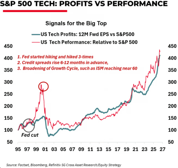
Both lines sit 50% above their 2000 peak — red near 430, teal near 420 — and that fact tells you almost nothing about whether we’re staring at the dotcom setup. The diagnostic was never the altitude; it was the gap. In March 2000, red decoupled to ~290 while teal stalled near 150 — a ~140-point chasm, performance running on pure multiple expansion while forward earnings refused to follow. Today the two lines track within a whisker. The rally is paid for, not borrowed: Nvidia’s data-center segment runs near a $35B quarterly clip, hyperscaler capex pushes toward a $400B combined run-rate, and each dollar of build lands on the counterparty’s ledger as signed RPO, metered cloud consumption, per-seat attach. That is contracted revenue, not pets.com eyeball counts. SocGen’s three preconditions confirm it — Fed hiking three times, spreads widening 6-12 months ahead, ISM near 60 — read zero of three: Fed cutting, spreads tight, ISM 54. Watch the spread, not the altitude. Red peeling above teal is the 2000 tell — until then, “higher than 2000” is geography, not pathology.
Market Intelligence Brief (MIB) Ver. 18.40
For professional investors only. Not investment advice.
© 2026 RecessionALERT.com