0.Change log

26 Sept 2024 : New Section-13 added to include “Job Losers” Sahm version. New Section-14 added “Performance summary”
28 Aug 2024  : New Section-6 added to include “Cycle Low” Sahm version. 

1.Introduction

In macroeconomics, the Sahm rule, or Sahm rule recession indicator, is a heuristic measure by the United States’ Federal Reserve for determining when an economy has entered a recession. It is useful in real-time evaluation of the business cycle and relies on monthly unemployment data from the Bureau of Labor Statistics (BLS). It is named after economist Claudia Sahm, formerly of the Federal Reserve and Council of Economic Advisors, who is accredited for creating the indicator.

The Sahm rule originates from a chapter in the Brookings Institution’s report on the use of fiscal policy to stabilize the economy during recessions. The chapter, written by Sahm, proposes fiscal policy to automatically send stabilizing payments to citizens to boost economic well-being. Instead of relying on human intuition to determine when such payments should be sent, Sahm outlines a condition to trigger the payments. The Sahm rule creates a 3-month moving average of the U.S unemployment rate and triggers a signal whenever this metric rises more than 0.5% from its low of the prior 12-months.

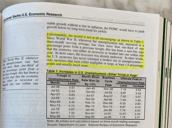
There is some debate about the naming of the rule, as many point out that it was first documented over 20 years ago by economist William C. Dudley in a Goldman Sachs research report, but where a lower trigger of 0.33% was suggested:

2.Performance

The chart below shows the performance of the metric both from a real-time observed (pre-revisions) and a post-revisions (hindsight observed) perspective. Small color-coded numbers represent the respective lag times in signalling actual starts in NBER declared recessions which are measured as the period following the business cycle peak through to the  trough:

We see that whilst the real-time and the hindsight versions regularly swap places in being earlier in signalling recession than the other, the real-time index gives slightly worse (higher lags) performance than the hindsight version. This means that looking at post-revised historical data (as most observers will be doing) the performance will look slightly better than is actually the case in real-time.

3.Smoothing

The use of a 3-month average of the unemployment rate for the Sahm rule calculation is unclear. It adds a significant lag to the recession-start signalling and for the historical period under review, only reduces one post-recession false positive from unsmoothed data from June 2003. It may well be that the lag is purposely introduced to optimise timing of citizen stabilizing payments or to eliminate risk of false positives & potential revision risks or to allow time for skills shortage (immigration)-driven unemployment (or other unemployment related aberrations not linked to a weak economy) to work through the system.

Until the reasoning for this 3-month smoothing becomes more clear, and even if it was deployed to eliminate the single June 2003 post-recession false-positive, we are inclined to use the un-smoothed unemployment rate in the SAHM calculation (“Unsmoothed-Sahm“) due to its superior timeliness (near-perfect coincident) in signalling recession starts. Even with the 10% false positive rate. At the very least, an unsmoothed-Sahm signal should be treated very seriously (90% confidence) even if we await the smoothed-Sahm for final confirmation some 2.5-3 months later. Furthermore, the false-positive can be ruled away when considering that the trigger only becomes active when the signal originates from zero within the last 12 months.

INCREDIBLE OFFER : Get 36% discount off our annual PRO Subscription, with macro- and market timing models plus unique in-depth quant research such as this research note. PLUS order before end of month and get a second year completely FREE. Get your discount HERE

4.Cycle Trough signalling

A lesser-known and unpublicized feature of the Sahm model is that both the standard averaged and unsmoothed Sahm versions are particularly useful in assessing recession ends through their definitive peaking motions (first fall when above +1.5) as demonstrated below where we have raised the y-axis to capture fuller range of motion:

It is very clear however that the unsmoothed-Sahm provides for near perfect coincident signalling of business cycle troughs whilst the standard Sahm is subject to 2-4 month lags.

5.Redux Versions

With our Redux #1 Sahm rule we can eliminate the 10% historic false-positive rate (single instance) with the unsmoothed-Sahm by raising the trigger threshold from 0.5 to 0.6, and still get superior signalling to the smoothed-Sahm. But given the false positive can be ruled-away (ignored if we dont originate from a low of zero), we feel this is unnecessary.

Best of all, our Redux #2 Sahm rule, uses a 7-month calculation window (as opposed to 12) with unsmoothed unemployment data to calculate the index. In this scenario each months unemployment rate is compared to the minimum of the prior 7 months as opposed to the prior 12 months. It eliminates the June 2003 false positive and has less false positive risk in general due to the muting effect of the 5-month shorter calculation window, whilst retaining near identical signalling (only 2001 changes from +0 to +2) of the unsmoothed version using the standard 12-month calculation window:

However, the Redux #2 Sahm rule signals recession-ends through peaking motions earlier than the standard unsmoothed Sahm, and has thus got inferior accuracy (absolute differences totaling 20 months vs 9 months) on this score, but these peaks provide extremely useful cues (early warnings) that the worst of the recession is likely over and a business cycle trough is on average 2 to 3 months away:

The ability to drop the calculation window down from 12 to 7 months without materially affecting signalling performance for the un-smoothed unemployment rate was interesting. Our research showed that we could drop the calculation window for the standard-Sahm from 12 to 9 months without impacting any recession signalling performance, but other than marginally better trough signalling performance, there would be no added benefits to doing so:

6.Cycle Low (Schannepp) Redux

The SAHM rule use the low of the last 12 months of their 3-month moving average of unemployment in their calculation with a 0.5 trigger. Whilst this one-size-fits-all rule works pretty well, we can improve on it by using the cycle low of the 3-month moving average (instead of the low of the last 12 months) with a lower trigger of 0.4. This is because some unemployment rate cycle lows can manifest more than 12 months before recessions start, namely January 1970 recession with 14 months, August 1990 recession with 16 months, January 2008 recession with 13 months and more recently 19 months ago from July 2024.

This methodology was first proposed in 2000 by Jack Schannep and is sometimes called the Schannep Recession Indicator. We show the Cycle Low version below, with the calculated indicator raised by 0.1 so it can share the same 0.5 trigger used by the Sahm rule in the below chart:

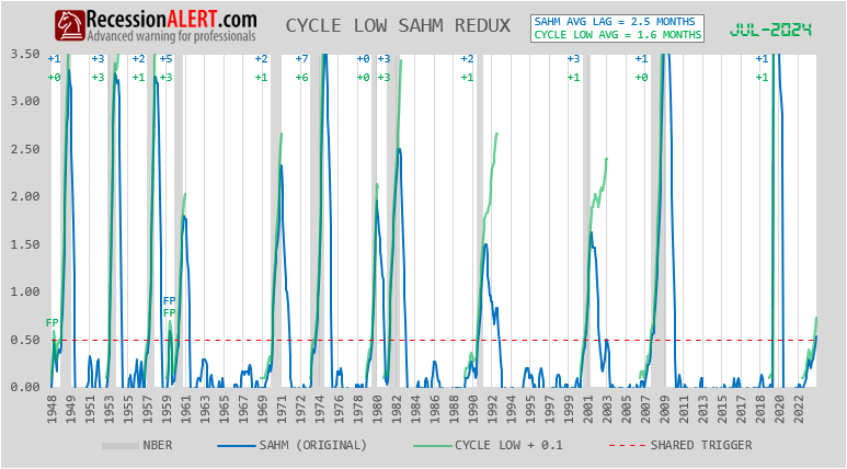
Quite clearly the average lag times to dating recessions of the Cycle Low rule are at least 0.9 month better than the standard Sahm rule (1.6 months versus 2.5 months). Whilst they share a false positive in 1959 however, the Cycle low version does have one extra false positive in 1948. Of the two, our opinion is that the Cycle low version is better despite the extra false positive.

7.Dataset fidelity

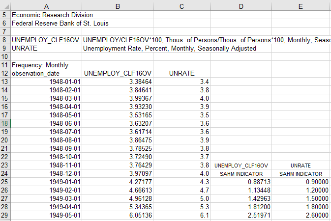
Most people deploy the standard nationwide unemployment rate (UNRATE in Fred) to the Sahm rule. But this is a rounded up number and only runs to one decimal. When you are using a trigger threshold of 0.5 on this dataset but its actually 0.45 rounded up then that can be quite a hefty margin difference. If you intent using unsmoothed Sahm indicators, its therefore probably better to calculate your own unemployment rate to at least two or three decimals using [UNEMPLOY (unemployment level) divided by CLF16OV (Labor force) times 100] to get numbers up to 5 decimals from FRED.

As shown below this results in data in the UNEMPLOY_CLF16OV column below versus the 1-decimal UNRATE. The difference it makes to the unsmoothed Sahm rule indicators (unemployment less low of prior 12 months) is shown in the last two columns and are rather substantial and can make the difference between a rule triggering or not. However, once you deploy 3-month moving averages suggested by the original Sahm rule, these differences become negligible and do not introduce any changes to triggers deployed at the 0.5% unemployment level.

8.Summary

The standard Sahm rule has a 3 month lag (on average) to NBER recession starts and a 1.3 month lag (on average) to recession ends. History has shown its signalling performance to be marginally affected by historical data revisions with zero false positives.

The unsmoothed Sahm rule has a 0.22 month lag (on average) to NBER recession starts and a near perfect identifications (zero lag) of recession ends, with a 90% confidence (1 post-recession false positive and 9 correct recession signals.) Deploying a rule that ignores triggers from signals that have not visited zero within the last 12 months rules-away the false positives.

For a 100% confidence (zero historical false positives), the Redux #2 Sahm rule has a 0.44 month lag (on average) to NBER recession starts and a 2-month lead to recession ends. It can provide useful warnings for when the unsmoothed Sahm is about to signal a recession end.

Dropping the standard Sahm calculation window from 12 to 9 months will preserve signalling with marginally improved lags and is thus not worth the effort.

Be cautious about data fidelity when calculating unsmoothed Sahm indicators.

INCREDIBLE OFFER : Get 36% discount off our annual PRO Subscription, with macro- and market timing models plus unique in-depth subscriber-only quant research such as this research note. PLUS order before end of month and get a second year completely FREE. Get your discount HERE

9.Sahm rule for U.S states

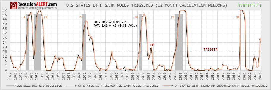
We can apply the Sahm rule to the monthly published unemployment-rate data for 52 U.S states and examine a diffusion (count) of U.S states that currently have Sahm rules triggered. We note from the chart below that due to the diffusion effect of the summing of 52 signals, the resulting lines are very smooth and there is zero benefit for running Sahm rules using the suggested 3-month moving average as this only serves to introduce a lag in the resulting diffusion (orange line below). For the purposes of further discussion we will thus only deal with unsmoothed Sahm calculations (black line below).

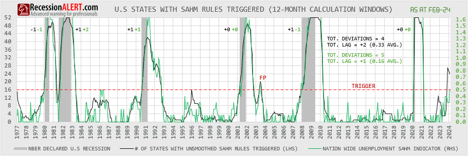
The chart below compares the State Sahm Diffusion with the standard unsmoothed nationwide unemployment Sahm indicator discussed in the beginning of this research, which has been scaled on the right axis so that the 0.5 trigger aligns with the 16-state threshold trigger. For all intents, the two mechanisms are identical, with the state-Sahm being marginally more accurate (4 versus 5 total sum of deviations) but with a slightly bigger average lag of 0.33 months versus 0.16 months:

Of particular interest however, is that the state Sahm indicator has flashed a recession signal four months ago (Nov 2023) whilst the nationwide unemployment Sahm sits on the cusp of a recession call.

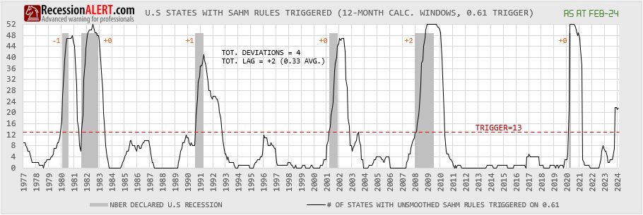
We can eliminate the 2003 false positive by triggering state Sahm rules on a rise in unemployment of more than 0.61% (as opposed to the standard 0.5%) from the prior 12-month lows, for a identical match in the total deviations (4) and average 0.33 month lag times to recession starts. This is the best zero-false-positive performance achievable from the state data when using a fixed trigger for the rise in unemployment across any calculation window:

The conclusion is that the best statewide Sahm rules model with a fixed one-size-fits-all trigger are matched in performance to the best unsmoothed national unemployment rate Sahm rules. Given the 52-fold increase in required data of the statewide models, its likely simpler to stick to the single-dimensioned unsmoothed national unemployment Sahm rules.

10.Individualized State Sahm rules

Since U.S states vary significantly in their populations and economies, a “one-size-fits-all” trigger for state Sahm models is likely too blunt an instrument. Many analysts publish smoothed state Sahm diffusions but the main problems with them are the smoothing (which introduces unnecessary lag in a diffusion model) and the one-size-fits-all rules. The employment and labour dynamics of each state are likely not a one-size fits all so it would make sense to have customized triggers for each state based on the profile of their respective Sahm indicators.

The author of the Sahm model, Claudia Sahm agrees that the 0.5% trigger was built for the national unemployment rate only and that it is better to look at individualized triggers if one were to build a state Sahm model.

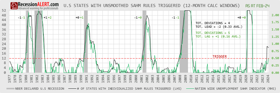
We examined each of the 52 states and set tailored trigger thresholds for each state that would maximise their recession signalling whilst minimising false positives. Individual states range from 0.4% to 1% Sahm triggers as a result. We can thus present a different “state individualized” model as shown below, which has been scaled on the right axis so that the 0.5 trigger of the original one-factor national Sahm model aligns with the new lower 12-state (as opposed to 16-state) diffusion threshold trigger:

This provides the best Sahm model of all, with zero false positives when considering sum total of recession start deviations (4) and average lead/lag to recession start. In this case the total deviations are identical between the individualized state model and the “one-trigger-size-fits-all” state model, but the individualized state model offer a 0.33 month average lead to recession as opposed to the 0.33 month average lag of the “one-trigger-size-fits-all” state model. This small improvement in earlier recession warning is what pushes the choice for the individualized state model slightly ahead of that of the “one-trigger-size-fits-all” state model and the unsmoothed single-factor Sahm model.

11.Sahm rules for U.S metros

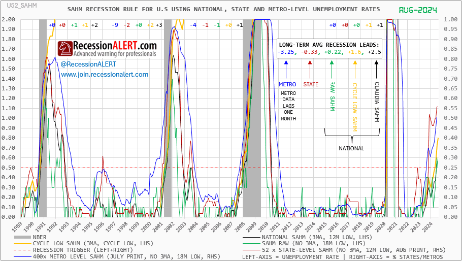
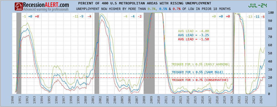
We can also apply Sahm rules to the 400 U.S metros for which the BLS compile unemployment data. This gives us greater granularity (400 as opposed to 52 data sets) and will also reduce the risk of a handful of states with any unemployment anomalies or large scale immigration overtly skewing the numbers. We also deploy multiple triggers for earlier warnings:

You will note we use 18-month lows in the calculations. We have found this threshold the best for when wanting to capture the full extent of unemployment degradation on a metro level. Whilst this means the post recession climbdowns of the indicators are lazy, the focus of this is on recession starts rather than on recessions end detection.

There are two downsides to this model however, namely the metro data publishing lags the state-data by one month and we only have history to 1990 (4 as opposed to 6 or more business cycles).

It is interesting to note that the 400-factor metro model, like the single-factor nationwide model – are not yet flagging recession as aggressively as the State model. This may point to immigration in a handful of states (which leads to temporary unemployment rises) may be skewing the odds toward recession in the state model and national models. Time will tell.

12.Showing it all together

Our subscribers get a monthly update on all the Sham Redux variants and state and metro versions in a single chart as part of the comprehensive monthly labor report we publish. It looks as follows as of July 2024, with the average leads/lags representative of the last 4 recessions shown on the chart.

13. Job Losers (U2) Redux

Despite the original Claudia Sahm variant now having joined all the other Sahm variants in issuing a recession warning, Claudia Sahm says the model will not correctly signal recession this cycle as there is no recession on the horizon.

Claudia Sahm points the blame on large scale immigration caused by strong economies that has attracted much needed immigration to meet the demands of a hot labor market. She makes a good point in a recent Bloomberg article that “According to the Congressional Budget Office, net immigration totaled 2.6 million in 2022 and 3.3 million in 2023, rising from an average of 900,000 a year from 2010 to 2019. As immigrants enter the economy, especially in large numbers, it can take them time to find work and thus raise unemployment rates.” 

Another factor to consider is that initial unemployment claims are not rising in tandem with the state-level unemployment gains – which again point to immigration as a potential suspect.

So the argument is that labor supply is increasing, raising the denominator of the unemployment rate equation and this is not a reflection of an economy performing poorly.

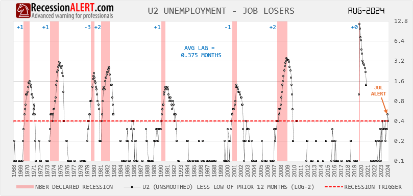
We can put this theory to the test in a number of ways. One of them is to look at the U2-Unemployment rate from BLS that tracks “Job losers and persons who completed temporary jobs, as a percent of the civilian labor force.” This is more a direct measurement of unemployment driven by the slowing economy as opposed to unemployment driven by increased labor supply:

There are four things to like about this measure:

1. It is less skewed by labor supply aberrations (immigration etc.)
2. It uses no smoothing or 3 month averages typical of national Sahm rules
3. It has zero historical false positives at the 0.4 threshold
4. It is far more timely at pinpointing recession starts than any other smoothed Sahm variant using U3 national unemployment data.

The one downside is U2 data is only available for the seven recessions since 1968 as opposed to Sahm variants using U3-unemployment data that goes back much farther.

The average lag of this model is 0.36 months, compared to +0.44 months for the Redux #2 Sahm rule, +1.6 months for the Cycle low rule and +2.5 months for the original Claudia Sahm rule.

The model shows there may be some truth to the labor supply issue as it shows a far less determined recession signal than the national Sahm models that look at traditional U3 unemployment ratios. However an alert was given in the July 2024 print which has since moderated again in the August print. But it definitely looks “touch and go”.

Our strategy is to monitor the original Sahm model, the unsmoothed model and Redux derivatives and the individualized state model together with the metro-level  and U2 models as a group to assess unemployment related recession risks. These models will be incorporated into our standard monthly Labor Report.

14.Performance Summary

Here is a tabular summary of the Sahm models covered so far in this research note, sorted by average NBER signalling lag:

At this point, considering signal lag to recession, false positives and length of historical data (sample size) available, it appears the U2-SAHM model offers the best performance for real-time recession detection, whilst the U3-State Sahm  provides best early warning.

INCREDIBLE OFFER : Get 36% discount off our annual PRO Subscription, with macro- and market timing models plus unique in-depth subscriber only quant research such as this research note. PLUS order before end of month and get a second year completely FREE. Get your discount HERE