Economic time series used in measuring business cycles and forecasting recessions are subject to revisions and re-benchmarking. Over time, more up-to-date and accurate data become available and time series are revised to reflect the updates. Some economic time series are subject to more drastic revisions than others. For example, the unemployment rate is subject to far smaller revisions than a broader time series such as GDP which is known to encounter very large revisions. Each instance of an update or revision to a time series is referred to as a “vintage”. Generally every time-series spawns a vintage on a weekly, monthly or quarterly basis depending on how often it is published.
When building leading or co-incident indices to measure business cycles and forecast recessions, the forecaster generally uses the latest vintage available and optimises his algorithms according to that. If the data he uses in his model is subject to large revisions he runs the risk that a current optimistic view of the indicator may very well turn out later to be a pessimistic one (or even the converse.) There is thus always this niggling concern about how much you can trust your models. As of June 2012, many forecasters are claiming we are in recession even though this view is not supported by many mainstream leading and co-incident indicators. Their claim is based on the fact that subsequent downward revisions will eventually show us in many months time that we were indeed in recession in the past.
To research and demonstrate the effects of data revisions and re-benchmarking on composite indices and recession forecasting, we took the “NBER Recession Model of last resort” which was constructed from July 2012 vintages of Industrial Production, Non-Farm payrolls, Personal Incomes and Retail Sales and rebuilt it using real-time data observations taken from the ALFRED Archival database of the Federal Reserve Bank of St Louis. This allows us to compare real-time observations of each of the 4 NBER Model components, as available to an outside observer at the time, to the latest August 2012 vintage. This will give us a feel for how significant the revisions are, especially around turning points just before and after NBER declared recessions . We then construct a real-time version of the weighted NBER composite co-incident economic index to see how revisions to its components effect recession forecasting.
About Growth Rates
You will recall from the NBER Model research note that we used different growth rate metrics for each of the 4 components of the model. These were not arbitrary selections, but those made to satisfy three criteria:
- The best pinpointing of recession starts and ends based on the vintage the model was built (the optimized model)
- The best pinpointing of recession starts and ends based on real-time observations (the real-time model)
- The smallest difference between (1) and (2) above
The last item is quite important as it is no use having a perfect optimized model that is markedly different to what we can expect from its real-time performance. Correct selection of growth rate in your model can indeed eliminate much of the issue associated with revisions. Although an economic time-series may have its levels revised downwards, if the recession models are using growth rates then its the impact of the revisions to growth rates that is important and not the levels themselves.
1. NON-FARM PAYROLL EMPLOYMENT (PAYEMS)
This is the first figure to be released, normally within the first week of the month. This component has the 2nd largest weighting (30%) in the NBER co-incident economic index, next to Personal Incomes which has a 31% weighting. We use a 3-month smoothed growth rate calculation for recession signalling, which uses data from the last 7 months observations in its calculations. The chart below shows the 3 month smoothed growth rate of the latest vintage of PAYEMS compared to that of the real-time observations an outside observer would have made with the latest vintage at his/her disposal at the time.
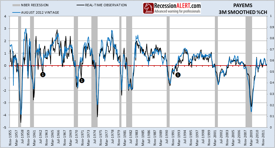
We observe several things from the above analysis. The first is that the real-time data results in several false positives (false alarms) as indicated by the “1” markings. These seem to be located soon after recessions though, and not before. The second observation is that for the most part, the signalling of the start of recessions by the revised data is slightly later than the real-time data, meaning the real-time observer would have been earlier in his/her assessment that a recession was indeed underway.
A detailed view of each of the past recessions is cataloged below with the real-time and revised (as of Aug 2012) Payroll time series. Green negative numbers in the bottom left corner of each chart show the lead that real-time observation has over revised data and red positive numbers show the lag that real-time observations has over revised data. We see that on average, the real-time observations of recession signals (when the data falls below zero) leads the revised data into recession by 1 month. Apart from this lead, there is no other discernible pattern with revisions for this data series.
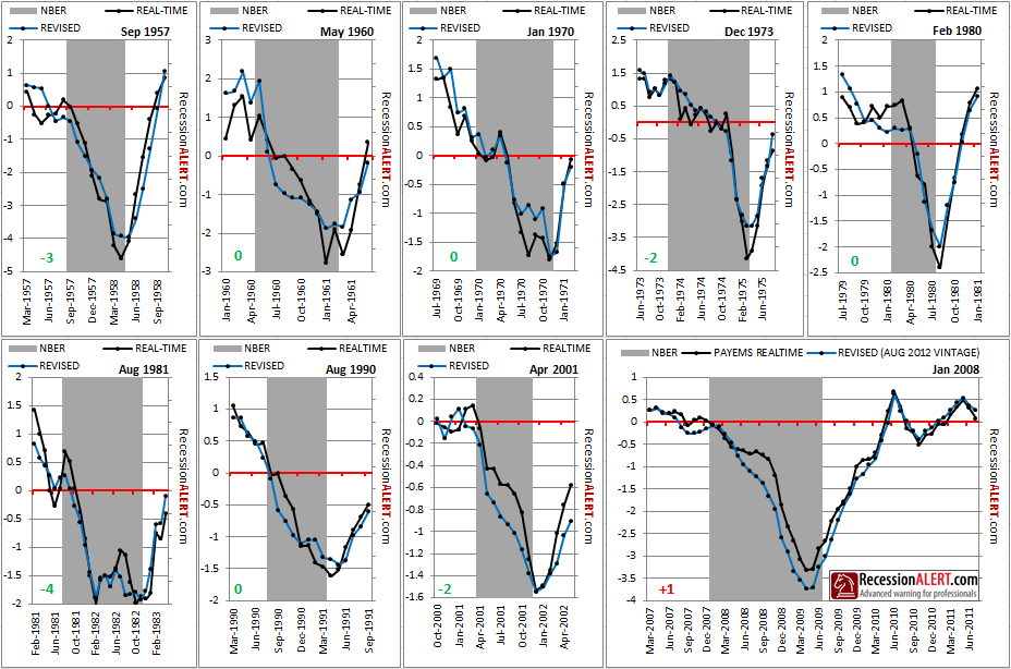
To conclude, whilst revised data results in a 3-month smoothed growth rate that can differ to that of the real-time growth rate, the larger differences seem to be isolated to the expansions and contractions, but not so much around the turning points themselves. We can expect the real-time data to provide 1 month average earlier warning than the revised data. Finally, PAYEMS revised and real-time growth rates can be significantly late in signalling recession as is evidenced by the 1960, 1970, 1973 and 1980 recessions. When being concerned about recession, revisions are not your problem with PAYEMS but occasional false positives and late signalling are.
2. REAL RETAIL SALES (RSAFS)
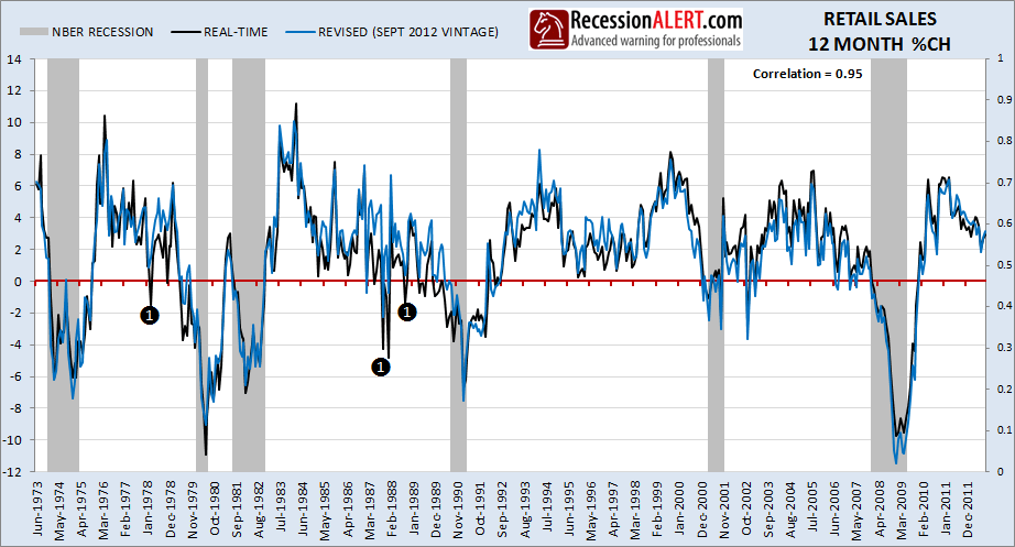
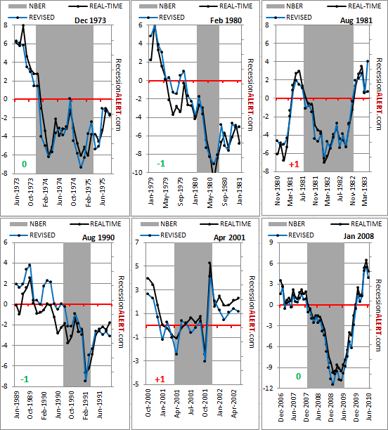
This is the second figure to be released, normally around the 14-15th of the month. This component has the smallest weighting (10.7%) in the NBER co-incident economic index. As this is quite a volatile series, we use a 12-month non- smoothed growth rate calculation for optimal recession signalling. The chart below shows the 12 month % growth rate of the latest vintage of RSAFS compared to that of the real-time observations an outside observer would have made. Note that the real-time vintage observations do not go back as far as PAYEMS, hence only 6 recessions are covered in this analysis.
We observe several things from the above analysis. The first is that the real-time data,as with PAYEMS, results in several false positives (false alarms) as indicated by the “1” markings. The second observation is that for the most part, the signalling of the start of recessions by the revised data is on average no sooner nor later than the real-time data. Again, as with PAYEMS, large differences between real-time and revised data do not seem to occur around business cycle turning points.
A detailed view of each of the past recessions is cataloged below with the real-time and revised (as of Aug 2012) Retail Sales time series. Green negative numbers in the bottom left corner of each chart show the lead that real-time observation has over revised data and red positive numbers show the lag that real-time observations has over revised data. We see that on average, the revised data and the real-time data have the same signalling of recessions when the growth rates fall below the red zero trigger line.
3. INDUSTRIAL PRODUCTION (INDPRO)
This is the third economic data set to be published for the NBER Model, normally a day or two after the Real Retail Sales data. It carries the third largest weight in the NBER model, at 16.7% of the co-incident index. We have found the 6-month smoothed growth rate, as defined by Prof Moore, to work the best for recession signalling and minimise the differences between real-time and revised data. The chart below shows the 6-month smoothed growth rate of the latest vintage of INDPRO compared to that of the real-time observations an outside observer would have made from published data available at the time.
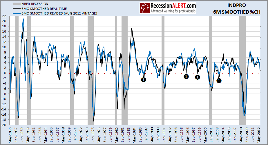
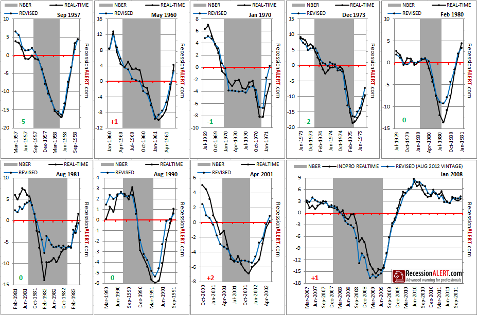
It is evident from the above chart that whilst large differences can exist between the revised and real-time growth observations, these differences are small around business cycle turning points. In fact, as the locations tagged with “1” show, your main concern with real time observations of INDPRO is not revisions, but false positives (flagging recession by dipping below zero, when there is no recession.) The detailed views of the past 9 recessions are below. Green negative numbers in the bottom left corner of each chart show the lead that real-time observation has over revised data into recession and red positive numbers show the lag that real-time observations has over revised data.
We see no discernible pattern from the effects of revisions when we are approaching recession. In 3 of the 9 cases, the real-time observations led the revised data into recession. In 3 of the 9 cases, the revised data led the real-time data and in 3 cases the revised and real-time observations concurrently fell into recession territory. However, on average, the real-time observations led the revised data by 0.4 months, predominantly due to the large lead it booked in the 1957 recession.

Comments are closed.