” The NBER does not define a recession in terms of two consecutive quarters of decline in real GDP. Rather, a recession is a significant decline in economic activity spread across the economy, lasting more than a few months, normally visible in real GDP, real income, employment, industrial production, and wholesale-retail sales.” – https://www.nber.org
Every month, we track the last 4 monthly items mentioned above in our “NBER Coincident Recession Model” which we publish for subscribers. These are affectionately known as the “Big Four” recession indicators and their data is made known on a monthly basis. Real-GDP (GDP deflated by the GDP implicit price deflater) and GDI is however published by the BEA on a quarterly basis, in the month following the end of the prior quarter. Each month thereafter it is re-published as re-estimations (so we have initial estimate, 1st release, 2nd final release.)
It is clear when reading various pronouncements made by the NBER Business Cycle Dating Committee that the two broadest measures of economic activity, real Gross Domestic Product (real GDP) and real Gross Domestic Income (real GDI) are very important in their determinations, probably more important than the Big-Four. The fact that these are only published quarterly is not an issue for them, since they can pronounce turning points up to 4 quarters later than when the event actually occurred.
In this research note, we investigate methods to utilise GDP and GDI in real-time to estimate recession probabilities in a timely fashion. These methods have resulted in a monthly “GDPI Report” we publish for subscribers which together with the monthly “NBER Model Report”, provide clients with a robust and timely method to follow all the components the NBER use in business cycle dating determinations. One of the great advantages of the quarterly GDP and GDI figures is that data is available going back to the post-war period, whereas a lot of monthly data is only available from the early 1960’s. This means recession models built with quarterly data are likely to be more robust and taken over many more recessions. A sample GDPI PDF report is available for one-click download right at the end of this research note.
1.GDP Background
GDP is supposed to represent the broadest measure of a nations’ economy. As is taught in introductory macroeconomics courses, it is possible to think of GDP in two different ways. One is as the dollar value of all final sales of goods and services produced by factors of production located within the United States (classic output-based GDP) and the second is as the dollar value of all the income generated by that production (Gross Domestic Income or GDI.)
The two measures are equal to each other by definition. But in practice, one can try to calculate GDP either using production data or using income data. If we obtain the production and income numbers from different sources, we’re certain to end up with different numbers for what is supposed to be the nation’s GDP. The difference between “gross domestic product” (GDP) and “gross domestic income” (GDI) is simply reported by the BEA as a “statistical discrepancy.”
The appeal of exploiting the information in GDI to date recessions is simple: it is as comprehensive as GDP, but it may capture information about the economy missed by measured GDP. Whilst most economists and business cycle analysts utilise classic real-GDP to determine recessions, several research papers have shown GDI deflated by the GDP deflater to be much more accurate at signalling recession starts in real-time. This is because GDI tends to weaken much faster in onset to recession than GDP, providing earlier signals.
The BEA release GDP one months after the quarter has ended whilst GDI for that quarter only gets published a month after that. Therefore a model that deploys both GDP and GDI for economy estimation is desirable from the point of timeliness.
All charts and models from this point on include data up to the 3rd quarter of 2012.
2.Building a GDP Recession Probability Model
The chart below shows real-GDP in relation to NBER defined recessions:
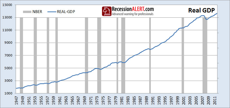
It appears from the above chart that for the most part, recessions occur when real-GDP dips. We can put this to the test by examining quarter-on-quarter growth rates of real GDP:
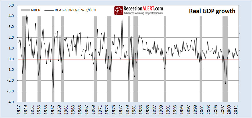
We note the occasional false positive (false alarm) when the rate of change dips below the red line and there is no recession, but we also note the occasional false negative (not showing recession when we are in one.) But on the whole this looks to be a pretty decent recession signal. Since quarter-on-quarter is the shortest possible growth rate we can look at, examining other, longer period growth rates should not achieve any additional benefits. This is indeed the case based on a battery of tests conducted by us and and so we will stick with this growth metric.
To get a really good feel for how well this growth metric serves in a recession probability model, we plugged it into a Probit model to display the following recession probability estimations:
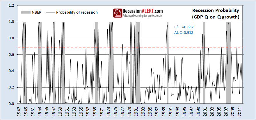
The Nagelkerke correlation coefficient of 0.667 shows a two-thirds correlation of the probability curve to the shaded NBER dates, whilst the Area-Under-Curve (AUC) of 0.918 shows the model correctly categorises the 260 quarters since 1947 into expansion and recession 91.8% of the time. The recession probability trigger is 0.7 (70% probability of recession) shown by the red dotted line. The false positives and negatives are shown clearly and the probability model is rather volatile, even during the course of robust expansions – not something we would like to use to make high-stakes calls.
In reality it’s hard to say from just one quarter’s value for GDP growth what is going on. Our research however has discovered that when including the prior quarters’ growth rate into the probability estimation (i.e. a 2 factor model as opposed to a single factor model), you can achieve a substantial improvement in the probability estimation model (using data further back than 1 quarter does not improve results):
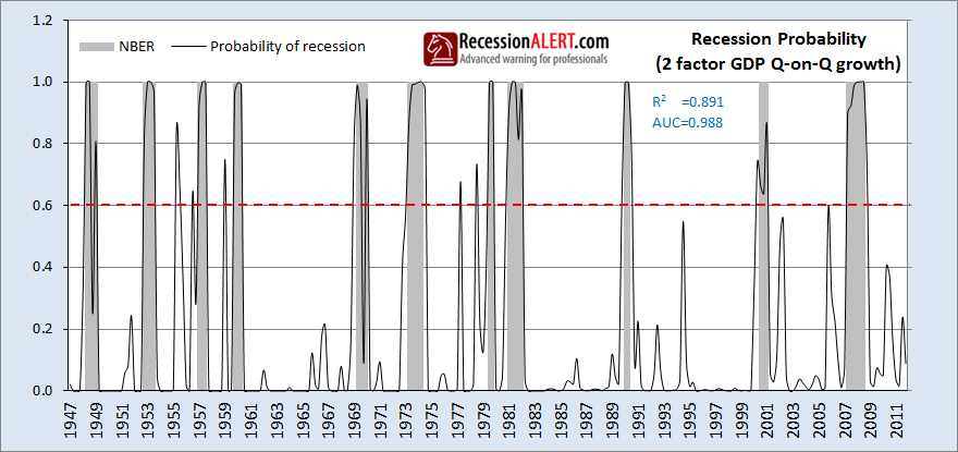
We observe substantial improvements in correlation and AUC and visibly you can see far less flaying about by the probability model which now has a bit more information on which to base its decision. We are also now able to lower our recession-call trigger from 0.7 to 0.6. We eliminated 2 false positives but introduced another for a net elimination of 1, but we substantially reduced the volatility (uncertainty) in the signal and eliminated 4 heart-stopping near-misses. Quite clearly, the prior quarters growth rate has a huge part to play in the estimation of recession when coupled with this quarters real-GDP growth rate.
This is now a robust model we can use, but not content with the outcome, our research uncovered that we could apply a non-parametric stylised trend-seeking approach to the real-GDP index, as described in detail in an older research piece we did “A Stylized Approach to Recession Forecasting” This means we can create a “Headwinds index” for real-GDP based on observations of its upward or downward movements over the last 6 quarters (we are not interested in the size of the movements, only the directions):
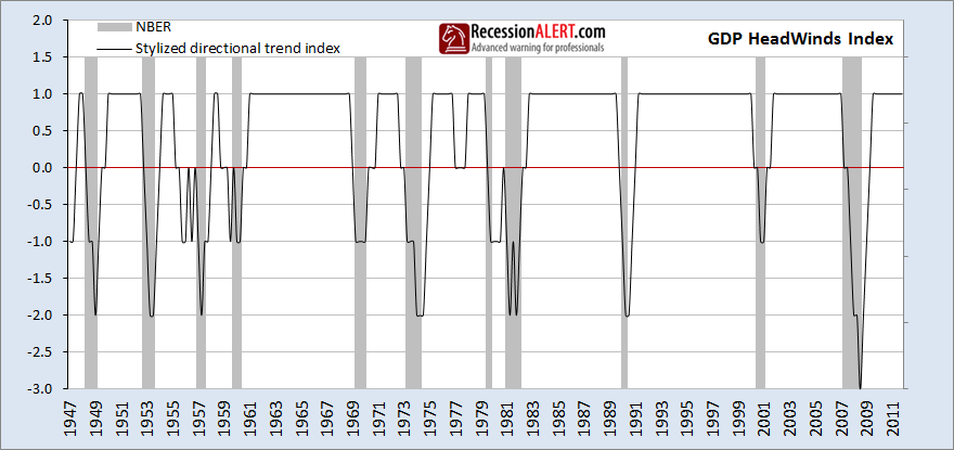
We note that this method is extremely good at the elimination of false positives (false alarms) and false negatives (when we are in recession it STAYS in recession) and it is much less likely to be affected by data revisions but as with everything there is a price to pay – as a discreet signal it aggregates a lot of informational content about the strength of smaller fluctuations of the economy in various states, seeking only to capture major trends up or down (cyclical Headwinds or Tailwinds) and it is somewhat slow in signalling the end of recessions. But its positives outweigh its negatives and it has important informational content to provide our recession probability estimation model as a 3rd factor:
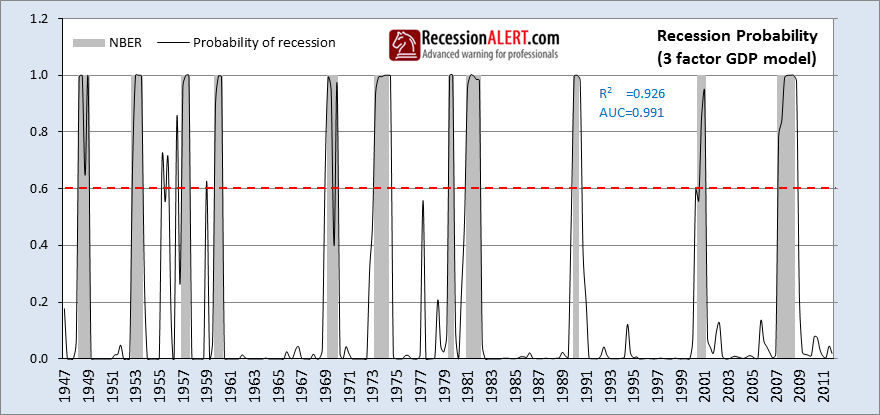
This remarkable 3-factor model eliminated 3 false positives, 1 false negative and 3 heart-stopping near-misses and has industrial strength correlation and AUC numbers.
3.Building a GDI Recession Probability Model
The chart below shows real-GDI (GDI deflated by the GDP price deflater) in relation to NBER defined recessions:
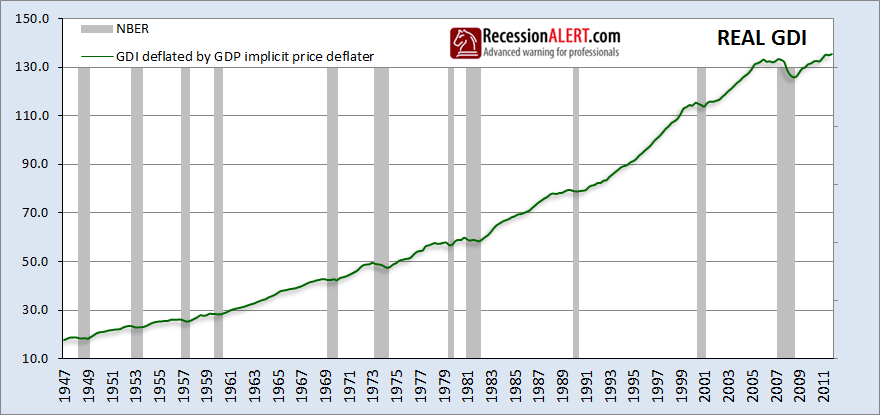
Again, as with real-GDP, downward trends seem to be directly related to periods of recession. As with GDP, we can put this to the test by examining quarter-on-quarter growth rates of real GDI:
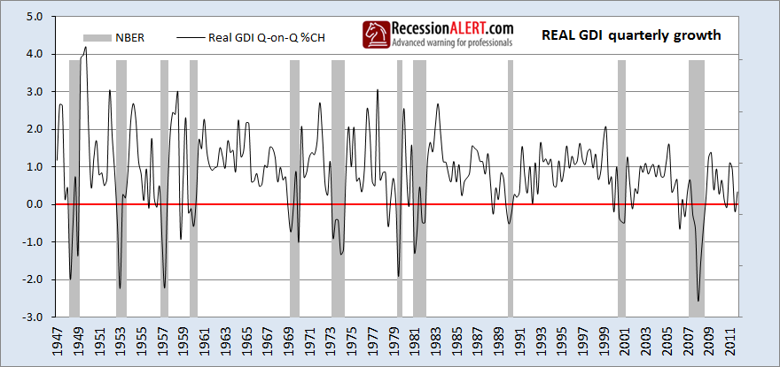
There are 2 less false positives with GDI and GDI growth signalled some recessions (especially the Great Recession) far earlier than GDP. Let’s have a look at the probability estimation model based on quarterly GDI growth to compare it to that of GDP:
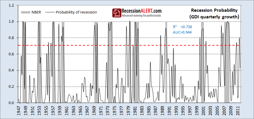
We see that the GDI quarter-on-quarter growth probability model provides better correlation to NBER than the GDP model (0.738 versus 0.667). It also provides a better AUC (0.944 versus 0.918). So we can quantitatively say that GDI provides better recession modelling than GDP. Note how GDI quarterly growth recently signalled recession.
Additionally, our research shows that the prior two quarters’ GDI growth rates also have recession recognition qualities when combined into a 3-factor probability model with the current quarters growth rate (remember that with GDP, only the prior quarters growth provided additional forecasting ability, so GDI seems to contain better informational content about the business cycle):
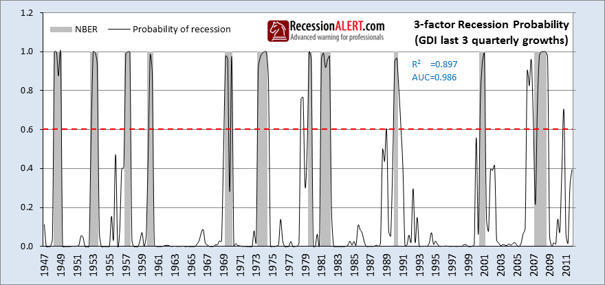
Again, just looking at quarterly growth rates, the GDI model provides slightly better correlation to NBER (0.897 versus 0.891) but has a marginally lower AUC than the GDP model (0.986 versus 0.988). However the greater historical informational content allows the GDI 3-factor model to post only 1 false positive in 1978 versus the GDP 2-factor models’ 5 false positives. Also, GDI has one false negative in the 1969 recession whereas GDP has two. This elimination of false positives and negatives is where the real power of GDI over GDP comes in with the quarterly growth models.
As with GDP, we discovered a highly favourable non-parametric, stylised trend-recognition algorithm for GDI which we combined into a GDI Headwinds Index:
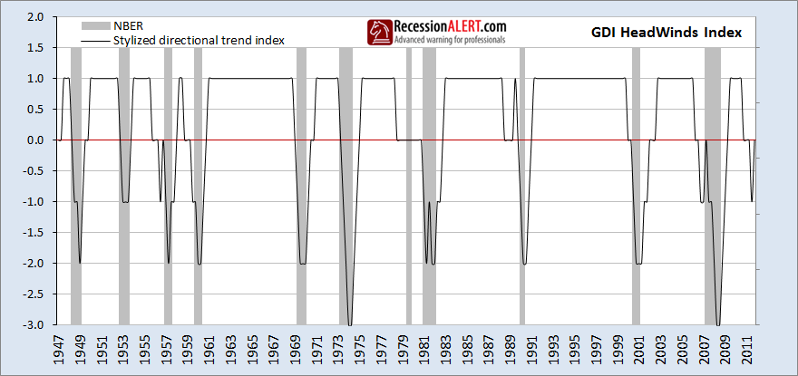
We can see that GDI negative trend momentum just before and during recessions is higher than that of GDP, with the GDI Headwinds frequenting -2 seven times and -3 twice versus the GDP headwinds that frequented -2 six times and -3 only once. It is very interesting (and disturbing) to note that GDI Headwinds placed a recession call in the 2nd quarter of 2012 (representing April, May , June) which seems consistent with the ECRI recession call. But this is just one factor in a multi-factor model so we would not advise panic just yet. Obviously the GDI Headwinds has forecasting ability to add to the recession model and this is borne out by the statistics in the 4-factor GDI recession probability model (using growth over the last quarter, and the same measurements from the prior two quarters, plus the Headwinds):
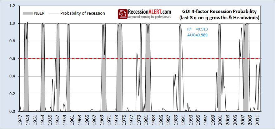
This provides a model that scores marginally less than the GDP 3-factor with an r-squared correlation of 0.913 (versus 0.926) and AUC of 0.989 (versus 0.991). However we have 1 false positive versus the GDP models 2. Also the GDI model did not signal a false negative in the 1969 recession as the GDP model did. It is also interesting to note how GDI picked up an early warning signal for the 2008 Great Recession, whereas the GDP model did not.
4. Combining GDP and GDI into a probability model
We have seen 3 factors from real-GDP and 4 from real-GDI that all have strong recession dating ability. The GDP and GDI multi-factor models are both industrial strength, and we would argue the GDI model has the slight edge over the GDP model due to less false positives and negatives. However, how about combining GDP and GDI into a 7-factor model so we have a very broad representation of the economy from both the output and the income side of the equation?
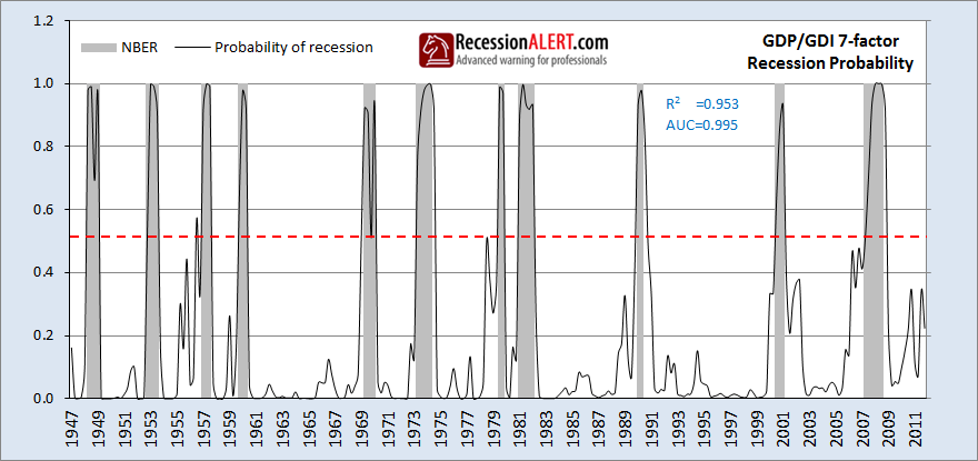
Bingo-the whole is greater than the sum of its parts with the 7-factor GDP/GDI model. If we discount the 1-quarter early signal in 1956 or alternatively move the trigger from 0.5 to 0.6, then we have a model with no false positives, no false negatives and very high r-squared and AUC numbers. In fact it is rare to see probability models with these kinds of statistics. The beauty of this model is that it is deploying two of the broadest measurements of the U.S economy possible, both from the output data and from the income data.
5. Combined GDP/GDI Economic Growth Model
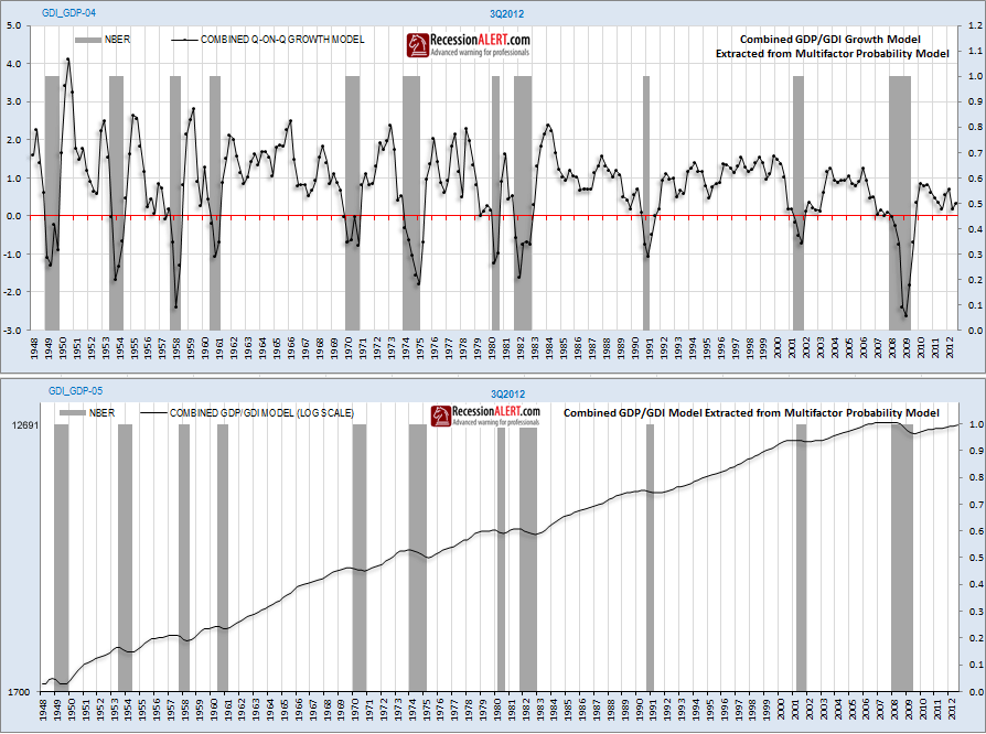
Using the 7-factor probability model that incorporates 3 factors from GDP and 4 from GDI, we can mathematically extract a new modified representation of the U.S production of goods and services that incorporates the output and the income side of the equation. Note that this is far more sophisticated than merely aggregating GDP and GDI together to achieve a dual-sided representation of output. We extract a month-by-month growth index (1st chart below) and a cumulative output index (2nd chart) below. These are more reflective representations of GDP for the U.S economy and include the benefits of both GDP and GDI into one index that most accurately describes business cycles since 1947:
6. Combined GDP/GDI Model Reports and Publishing
Although GDP and GDI are published quarterly, they are revised each month. Additionally we incorporate monthly estimations for GDP and GDI to carry us between quarterly GDP/GDI prints to give us a more real-time view. For this reason we update the report every month and publish it in the first week of every new month. The report is available to PRO ($349 per annum) subscriptions only and a new tab has been made available for it next to the NBER Model tab in the MEMBERS download section of our web site.

To download a sample copy of the report dated to 3rd quarter 2012 , click on the below image:


Comments are closed.